Fact Finding: Simplifying the Circuit (Post 2)

post by Senthooran Rajamanoharan (SenR), Neel Nanda (neel-nanda-1), János Kramár (janos-kramar), Rohin Shah (rohinmshah) · 2023-12-23T02:45:49.675Z · LW · GW · 3 comments

Contents

  Introduction
  Set-up
  The simplified circuit that we ended up with
  Investigation 1: Understanding fact extraction
    Which nodes contribute most to the output logits?
    To where do these high-effect heads attend?
    What are these high-effect attention heads reading from the final name token position?
    A simplified subcircuit for fact extraction
    An Alternate Path: Just Train A Linear Probe
  Investigation 2: Simplifying de-tokenization and lookup
    Lookup is mostly complete by layer 6
    Context doesn’t matter when looking up an athlete’s sport
    Attention heads don’t matter beyond layer 2
    A simplified subcircuit for fact lookup
  Investigation 3: Further simplifying the token concatenation circuit
    Token concatenation is achieved by attention heads moving token embeddings
    For two-token athletes, concatenate_tokens literally adds first and last name tokens together
None
3 comments

This is the second post in the Google DeepMind mechanistic interpretability team’s investigation into how language models recall facts [? · GW]. This post focuses on distilling down the fact recall circuit and models a more standard mechanistic interpretability investigation. This post gets in the weeds, we recommend starting with post one [AF · GW] and then skimming and skipping around the rest of the sequence according to what’s most relevant to you. We assume readers of this post are familiar with the mechanistic interpretability techniques listed in this glossary.

Introduction

Our goal was to understand how facts are stored and recalled in superposition. A necessary step is to find a narrow task involving factual recall and understand the high level circuit that enables a model to do this task.

We focussed on the narrow task of recalling the sports played by different athletes. As discussed in post 1 [AF · GW], we particularly expected facts about people to involve superposition, because the embeddings of individual name tokens is normally insufficient to determine the sport, so the model must be doing a boolean AND on the different tokens of the name to identify an athlete and look up their sport. Prior work calls this phenomenon ‘detokenisation’ and suggests it involves early MLP layers, and uses significant superposition.

Why focus on athletes’ sports rather than factual recall in general? We believe that in mechanistic interpretability, it’s often useful to first understand a narrow instance of a phenomenon deeply, rather than insisting on being fully general. Athletes’ sports was a nice task that gave us lots of examples per attribute value, and our goal was to understand at least one example where superposition was used for factual recall, rather than explaining factual recall in general. We conjecture that similar mechanisms are used for recalling other classes of fact, but this wasn’t a focus of our work.

Set-up

To understand fact localisation, we studied Pythia 2.8B’s next token predictions and activations for one-shot prompts of the form:

For 1,500 athletes playing the sports of baseball, basketball and (American) football. To choose these athletes, we gave the model a larger dataset of athletes from Wikidata and filtered for those where the model placed more than 50% probability on the correct sport^[1].

We chose Pythia 2.8B as it’s the smallest model that could competently complete this task for a large number of athletes.

We made the prompts one-shot because this significantly improved the model’s performance on the task^[2]. We chose golf for the one shot prefix so that the model didn’t have a bias towards one of the three sports it needed to predict. For simplicity, we didn’t vary the one shot prefix across the prompts.

The simplified circuit that we ended up with

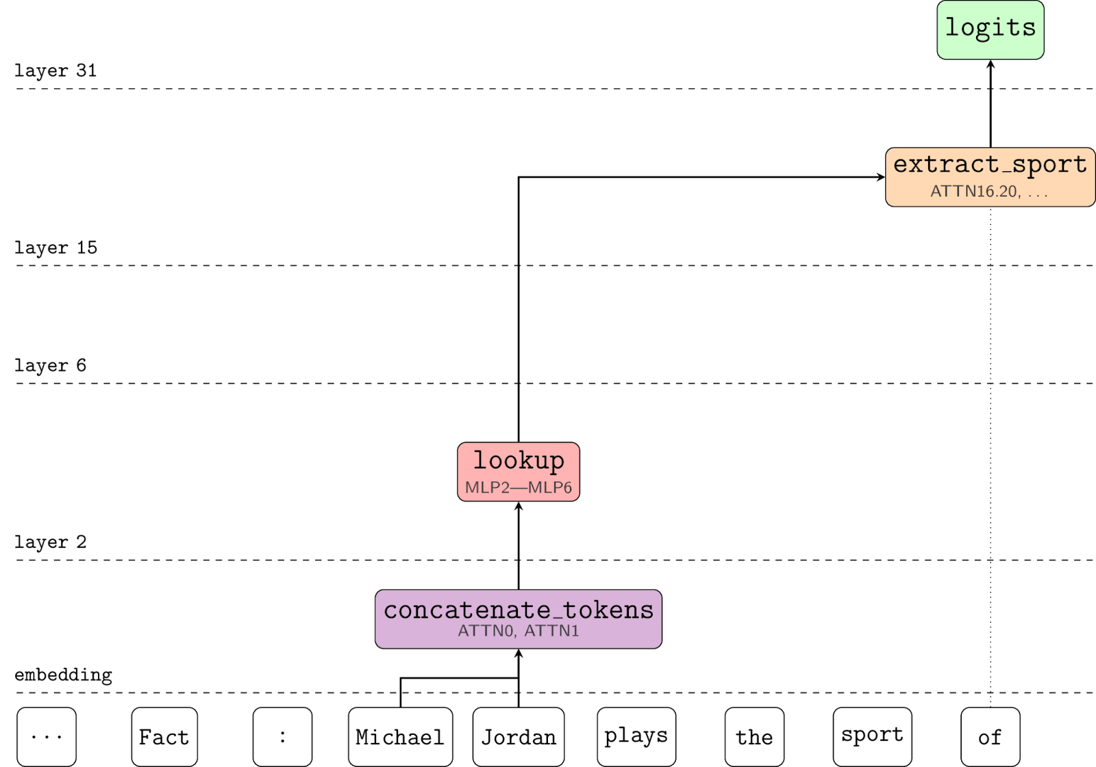
Before going in detail through the ablation studies we performed to derive the circuit, let’s take a look at the simplified circuit we ended up with:

Where:

• concatenate_tokens performs something roughly like a weighted sum of the individual token embeddings, placing each token’s embedding in a different subspace, implemented by the first two layers of the model;^[3]

• lookup is a five layer MLP (whose layers match MLP layers 2 to 6 in the original model)^[4] that processes the combined tokens to produce a new representation of the entity described by those tokens, where this representation can be linearly projected to reveal various attributes about the entity (including the sport they play);

  • We note that in the path from layer 6 to layer 15 there seem to be multiple MLP layers that matter, but we believe them to mostly be signal boosting an existing linear representation of the sport, and ablating them does not significantly affect accuracy.

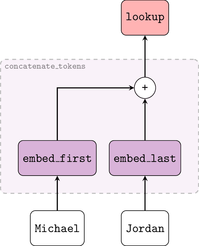
• extract_sport is a linear classifier that performs an affine transformation on the representation generated by lookup to extract the sport logits that are returned by the model. This is implemented in the model by several attention heads (notably including L16H20) which attend from the final token to the final name token and directly compose with the unembedding layer^[5]. In the special case of athletes whose names only consist of two tokens (one for the first name, one for the last name), we were able to further simplify the concatenate_tokens function to be of the form:

Where embed_first and embed_last are literally lookup tables (with one entry per token in the model’s vocabulary) with disjoint ranges (so that the encoder can distinguish “Duncan” the first name from “Duncan” the surname) – reinforcing the idea that the result of concatenate_tokens is only as linearly informative as the individual tokens (plus positional information) themselves – i.e. it is a dense / compressed representation of a related sequence of tokens that the model needs to decompress / extract linear features from in order to be usable by downstream circuits (such as extract_sport).^[6]

This is fairly consistent with prior work in the literature, notably Geva et al. We see our narrow, bottom-up approach as complementing their broader and more top down approach to understanding the circuit. We further show that extract_sport is a linear map, mirroring Hernandez et al, and that it can be understood in terms of the OV circuit of individual attention heads. We see our contribution as refining existing knowledge with a more bottom up and circuits focused approach in a narrow domain, and better understanding the model’s representations at each stage, rather than as being a substantially new advance.

In the remainder of this post, we describe in further detail the experiments we performed to derive this simplified circuit.

Investigation 1: Understanding fact extraction

When the model outputs the correct sport token to complete the prompt, where is the earliest token at which the sport was determined? Prior work suggests that the correct sport should be identified early on in the sequence (at the athlete’s final name token) and placed in a linearly recoverable representation. A separate fact extraction circuit (extract_sport in the circuit diagram above) would then read the sport from the final name position and output the correct logits to complete the prompt.

In this section, we describe the experiments we performed to verify that this picture holds in reality and to identify the circuit that implements this fact extraction step.

Which nodes contribute most to the output logits?

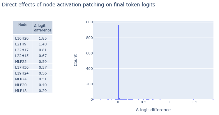
We started off by identifying which nodes in the model have the greatest direct influence on the logits produced at the final token. We did this by individually ablating the activations for each MLP layer and attention head output at the final token position and measuring the direct effect on the output logits.

Specifically, for each clean prompt and each node we wished to ablate, we would take activations for that node from a “corrupted” prompt and patch these into the activations for the clean prompt just along the patch connecting that node to the model’s unembedding layer, in order to measure the effect of this path patch on the model’s outputs. For the corrupted prompt, we would randomly pick a prompt for an athlete who plays a different sport.^[7] To measure the direct effect, we would compare the logit difference between the clean prompt’s sport and corrupt prompt’s sport, before and after path patching.^[8] The results are as follows:

These results show that a relatively sparse set of nodes have any meaningful effect on the logits:

• A handful of attention heads in the mid-layers;
• The MLP layers that follow these attention heads.

Of these, the attention heads are particularly interesting: since we have measured direct (not total) effect, we know that the outputs of these attention heads are directly nudging the final tokens logits towards the correct sport (or away from incorrect sports), without the need for further post-processing.^[9] This strongly suggests that, wherever these heads are attending to, the residual stream at those locations already encodes each athlete’s sport.

To where do these high-effect heads attend?

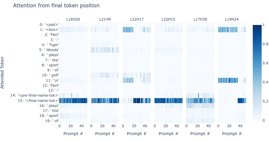
Here, we’ve visualised the attention patterns from the final token over a sample of prompts for the 6 heads with the highest direct effect on the final token logits. We see that the heads mostly attend either to the final name token position or, failing that, look back to either the “<bos>” or “\n” resting positions earlier in the prompt.^{[10] [11]} From this we can conclude two things:

1. An athlete’s sport is largely represented in the residual stream by layer 16 of their final name token.
2. The representation of their sport should be linearly recoverable (because each head’s value input is related to the model’s final token logits by an approximately linear transformation).

What are these high-effect attention heads reading from the final name token position?

To answer this question, we computed the path-specific effects of nodes in the final name token position via the OV circuits for each of the high-effect heads listed above. To be precise, for each high-effect head, we path patched, one by one, each feeder node’s activation on the corrupted (other-sport) prompt along just the path from that node to the output logits via the relevant head’s OV circuit^[12]. In effect, this creates an attribution of each high-effect node’s value input in terms of the nodes that feed into it.

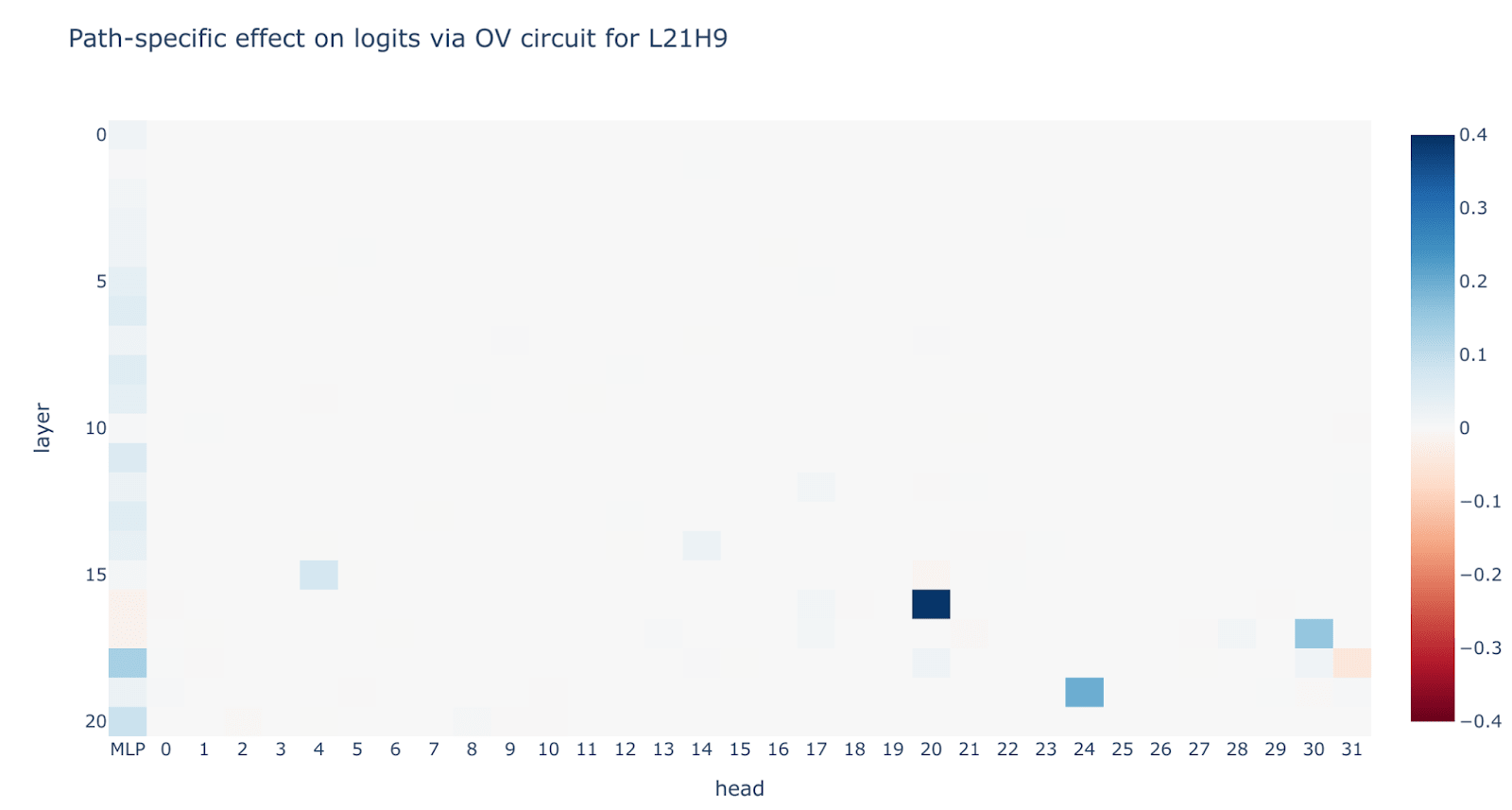
Interestingly, we found that a large part of the second to sixth most important heads’ performance comes in turn from their value inputs reading the output of L16H20 at the final name token stream. For example, here is the attribution for final name token nodes’ impact on the logits via the OV circuit for L21H9 (the second most important head) – note the outsized contribution of L16H20’s output (at the final name token position) on the effect of this head:

The heatmaps for the third to sixth most important heads looked similar, with a lot of their effect coming from the output of L16H20 at the final name token.

Furthermore, looking at the attention patterns for L16H20 when attending from the final name token position, we see that it typically attends to the same position. Putting these observations together, we see that L16H20 has a high overall importance in this circuit through two separate mechanisms:

1. It transfers the athlete sport feature directly to the final token position via its OV circuit (attending from the final token back to the final name token);
2. It attends from the final name token position to the same position, producing an output that significantly contributes (via V-composition) to the outputs of other heads that transfer the athlete sport feature from the final name token to the final token.

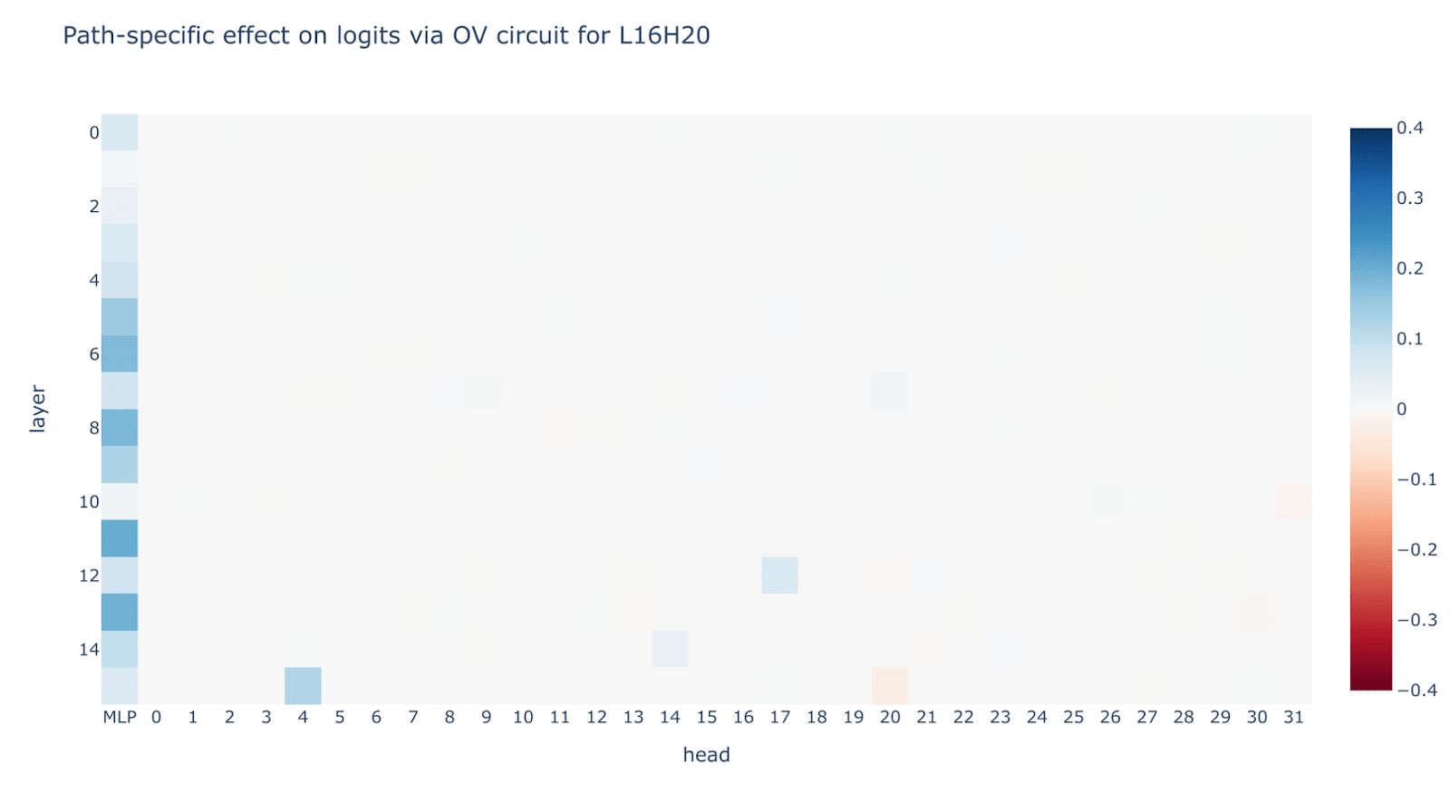
What about L16H20 itself – which nodes most strongly contribute to its value input? As the chart below shows, the value input for L16H20 itself is largely dependent on MLP outputs preceding it in the final name position (with some V-composition with a handful of earlier heads that in turn attend from the final name position to itself):

A simplified subcircuit for fact extraction

Putting the above results together, we conclude that:

• A large part of the sport fact extraction circuit (extract_sport in the diagram above) is performed by head L16H20;
  • Because the head’s attention pattern does not change (much) between athletes, its function is just a linear map, multiplying the residual stream by its OV circuit.
• This head’s OV circuit reads the final name token residual stream and outputs the contents (both back into the same residual stream and directly into the final token residual stream) such that unembedding the result boosts the logits for the correct sport’s token over those for incorrect sports’ tokens.
• Therefore the correct sport was linearly represented on the final name token, and extracted by L16H20’s OV circuit.

This suggests we can approximate extract_sport by replacing all of the model’s computation graph from layer 16 at the final name token position onwards with a three-class linear probe constructed by composing the OV map for L16H20 with the model’s unembedding weights for the tokens “ baseball”, “ basketball” and “ football”.^[13]

Making this simplification, we find that the overall circuit’s accuracy at classifying athlete’s sport drops from 100% for the original model, to 98% after simplifying the extract_sport part of the circuit to this (weights-derived) linear probe – i.e. we can vastly simplify this part of the circuit with negligible drop in performance at the task.^[14][15]

An Alternate Path: Just Train A Linear Probe

An alternate route that short-cuts around a lot of the above analysis is to just train a logistic regression probe on the residual stream of the final name token^[16] and show that by layer 6 the probe gets good test accuracy. We could further show that patching in the subspace spanned by the probe^[17] causally affects the model’s output, suggesting that the representation is used downstream^[18]. This was the approach we used for a significant part of the project, before going back and making the analysis earlier in this section more rigorous.

We think there are significant advantages of mechanistic probes (e.g. using the weights of L16H20 and the unembedding to derive a probe rather than training a logistic regression classifier), it’s more principled (in the sense that we can clearly see what it means in terms of the model’s circuits), harder to overfit, and doesn’t require a training set that can then no longer be used for further analysis. But “just train a probe” makes it easier to move fast.

In particular, for this investigation, our goal was to zoom in on lookup in the first few layers, and knowing that the correct sport became linearly represented after a couple of MLP layers sufficed to tell us there was something interesting to try reverse-engineering, even if we didn’t know the details of the fact extraction circuit.

We think that probes are an underrated tool for circuit analysis, and that finding interpretable directions/subspaces in the model, which can be shown to be causally meaningful in a non-trivial way, enables simpler circuit analysis that needs only consider a subset of layers, rather than the full end-to-end behaviour of the model.

Another simpler approach would be to search for a mechanistic probe by just iterating over every head, taking its OV times the unembedding of the sports as your probe, and evaluating accuracy. If there’s a head with particularly high accuracy (including on a held-out validation set) that attends to the right place, then you may have found a crucial head. We note this approach has more danger of overfitting, depending on the number of heads, than doing a direct logit attribution first to narrow down to a small set of heads^[19].

Investigation 2: Simplifying de-tokenization and lookup

In this section we describe the experiments we performed to simplify the part of the circuit covered by the concatenate_tokens and lookup modules as defined in the simplified circuit diagram above. To summarise, the experiments described below establish the following facts about this part of the circuit:

• An athlete’s sport is represented much earlier in the residual stream than layer 16 (where it is read by head L16H20). By layer 6, we still get pretty good (90%) accuracy when trying to read athlete’s sports using extract_sport.
• Context prior to the athlete’s name doesn’t matter for producing the sport representation (though it does matter for extract_sport). We can use the model’s final token activations on prompts of the form “<bos> <athletes-full-name>” and extract the athlete’s sport with little drop in accuracy.
• Attention heads don’t matter beyond layers 0 and 1. We can mean-ablate attention layers 2 onwards without hurting the lookup module’s performance much. Looking at attention patterns, we see that most heads do not particularly attend to previous name tokens, strengthening the case for ablating them. The advantage of removing these attention heads is that the lookup module thus becomes a simple stack of MLP layers (with residual skip connections) that is able to take the athlete’s embeddings at the start of layer 2 in the residual stream and output the athlete’s sport by the end of layer 6 in the residual stream.

As a result, we can decompose this part of the circuit into two sub-modules:

• concatenate_tokens, representing the role of layers 0 and 1 of the model, whose role (for this task) is to collect the athlete’s name tokens and place them in the final name token residual stream (we show in Investigation 3 that this is pure concatenation without lookup, at least for two token athlete names);
• lookup, a pure 5-layer MLP (comprising layers 2–6 of the original model) that converts this multi-token representation of the athlete’s name into a feature representation of the athlete that specifically represents the athlete’s sport in a linearly recoverable fashion.

We now describe the evidence supporting each of the three claims listed above in turn.

Lookup is mostly complete by layer 6

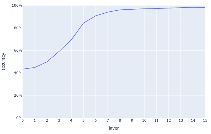
If we apply the extract_sport probe to different layers in the final name token position, we see that it’s possible to read an athlete’s sport from the residual stream much earlier than layer 16:^[20]

By around layer 8, accuracy has largely plateaued, and even by layer 6 we have about 90% accuracy.^[21]

Context doesn’t matter when looking up an athlete’s sport

We have already established that the residual stream at the final name token for an athlete encodes their sport. But to what extent did the model place sport in the residual stream because it would have done this anyway when seeing the athlete’s name (the multi-token embedding hypothesis) and to what extent did the model place sport in the residual stream because the one-shot prompt preceding the name^[22] hinted to the model that sport might be a useful attribute to extract?

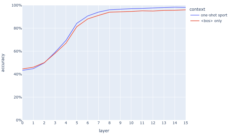
Our hypothesis was that the context wouldn’t matter that much – specifically that the model would look up an athlete’s sport when it sees their name, even without any prior context. We tested this by collecting activations for pure name prompts, where the model was fed token sequences of the form “<bos>^[23] <first-name> <last-name>”^[24] and the residual stream was harvested from the final name token.

Can the extract_sport module read athletes’ sports from these activations? As the plot below shows, we found that there is a little drop in performance without the one-shot context, but it’s still possible to fairly accurately read an athlete’s sport purely from an early layer encoding of just their name prepended by “<bos>”, without any additional context. Hence, we can simplify the overall circuit by deleting all edges from tokens preceding the athlete’s name tokens in the full prompt for the task.

Attention heads don’t matter beyond layer 2

In order to recall sport accurately, the lookup part of the circuit must in general be a function of most (if not all) of the tokens in an athlete’s name: for most athletes, it’s not possible to determine sport by just knowing the last token in their surname. Hence, attention heads must play some role in bringing together information distributed over the individual tokens of an athlete’s name in order that facts like sport can be accurately looked up.

However, how do these two processes – combining tokens and looking up facts – relate to each other?

1. They could happen concurrently – with attention bringing in relevant information from earlier tokens as and when it is required for the lookup process;
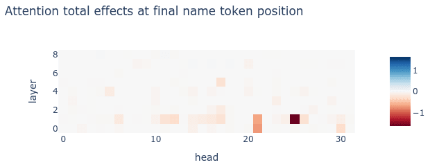
2. Or the processes could happen sequentially, with the tokens making up an athlete’s name being brought together first, and much of the lookup process only happening afterwards.^[25] Looking at the total effects of patching attention head outputs at the final name token position, we did find that there are many more heads that play a significant role in the overall circuit in layers 0 and 1 of the model than in later layers:

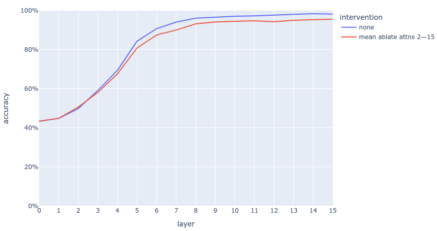
This suggested that we might be able to remove the attention head outputs for layer 2 onwards without too much impact on the overall circuit’s performance. Trying this, we found that mean ablating attention outputs from layer 2 onwards had only a slightly detrimental impact on accuracy:^[26]

This supports the two-stage hypothesis described above: information sharing between tokens (via attention) is largely complete by layer 2, with attention heads in later layers unimportant for lookup.

A simplified subcircuit for fact lookup

The results above suggest that we can indeed split the process of looking up an athlete’s sport into two stages:

• concatenate_tokens, which is the result of the embedding and layers 0 and 1 of the model processing the tokens comprising the athlete’s name^[27] and producing a “concatenated token” representation at the end of layer 1 in the final name token residual stream;

• lookup, which is a pure MLP with skip connections (made up from MLP layers 2 onwards in the model), which processes the “concatenated token representation” after layer 1 of the residual stream, which in itself poorly represents the athlete’s sport (in a linear manner), and produces a “feature representation” later on in the residual stream, where sport can be easily linearly extracted (by sport_extract).

Note that there are two simplifications we have combined here:

• Processing the athlete name tokens on their own without a one-shot prompt (because we found context to be unimportant)
• Removing attention heads from layer 2 onwards (because we found information transmission between tokens to largely be complete by layer 2).

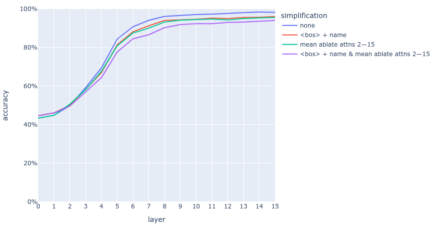
Since, each of these approximations has some detrimental effect on the circuit’s accuracy, it’s worth assessing their combined impact. Here’s a plot showing how combining these approximations impacts accuracy:

The upshot is that, even applying both simplifications together, it’s possible to get up to 94% accuracy by including enough layers in the lookup MLP; even stopping at layer 6 gets you 85% accuracy.

Investigation 3: Further simplifying the token concatenation circuit

So far, we have:

• Simplified extract_sport to a 3-class linear probe, whose weights are derived by composing the OV map for L16H20 with the model’s unembedding weights;
• Simplified lookup to be a pure 5 layer MLP with skip connections, whose layer weights correspond to those of MLP layers 2–6 in the original model;
• Established that prior context can be removed when calculating the residual stream’s value at the beginning of layer 2 at the final name token position (which is the input for lookup).

This leaves us with concatenate_tokens, comprising the embedding and layers 0 and 1 of the model, which converts the raw athlete name tokens (plus a prepending <bos> token) into the value of the residual stream at the beginning of layer 2. Can we simplify this part of the circuit further?

There are two levels of simplification we identified for this components of the circuit:

• In general, we can think of concatenate_tokens as effectively generating two separate token-level embeddings of the athlete’s name, and then combining these embeddings approximately linearly via pure attention operations;
• In the case of athletes whose names are just two tokens long, we can further approximate concatenate_tokens so that it is literally a sum of effective token embeddings for first and last name tokens, taking only a modest hit to circuit accuracy.

In the following subsections, we explain these simplifications in more detail and provide experimental justifications for them.

Token concatenation is achieved by attention heads moving token embeddings

The first simplification comes from the following two observations:

• MLP layer 1 at the final name token position has little importance for circuit performance: resample ablating it has low total effect on logit difference for the original model, and mean ablating it has little impact on the accuracy of the simplified circuit.^[28]

• Due to Pythia using parallel attention, MLP layer 0 is effectively a secondary token embedding layer.^[29] This implies that (after mean ablating MLP 1), concatenate_tokens effectively performs the following operations:

1. Calculate primary token embeddings for the athlete name tokens (and <bos>) using the model’s embedding layer weights.
2. Calculate secondary token embeddings for the athlete name tokens using the embedding weights induced by the action of MLP 0 on the input token vocabulary.
3. Operate the attention layer 0 heads on the primary token embeddings.
4. Operate the attention layer 1 heads on the sum of the primary token embeddings, secondary token embeddings and outputs of attention layer 0.
5. Use the result of step 4 at the final name token position as the input to lookup.

In other words, concatenate_tokens effectively embeds the input tokens (twice) and moves them (directly and indirectly) to the final name token position via attention.

For two-token athletes, concatenate_tokens literally adds first and last name tokens together

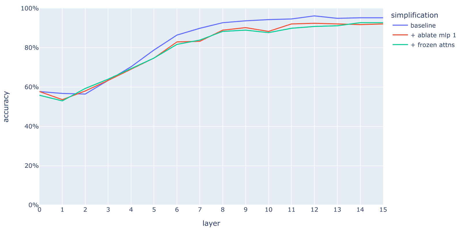
For two-token athletes, we found that we could furthermore freeze attention patterns and still retain reasonable accuracy on the task. Specifically:

• We prevented attention heads in layer 1 at the last name token position attending to the same position;
• We froze all other attention patterns at their average levels across all two token athletes in the dataset, making the attention layers just act as a linear map mapping source token residuals to the final token.

These simplifications, along with mean ablating MLP 1, turn concatenate_tokens into a sum of effective token embeddings and a bias term (originating from the embeddings for the <bos> token). The effective token embedding of the last name is just the sum of the primary and second (MLP0) token embedding. The effective token embedding of the first name is more complex, it’s the primary token embedding times the linear map from frozen attention 0 heads (their OV matrices weighted by the average attention from the last name to the first name), plus the primary and secondary token embeddings times the linear map from frozen attention 1 heads.

The impact of these simplifications on accuracy are shown in the graph below.^[30] We see that, for two-token athletes, freezing attention patterns has little additional impact on accuracy over ablating MLP 1.

---

1. Note that we started with several thousand athletes, so this filtering likely introduced some bias. E.g. if there were a thousand athletes the model did not know but guessed a random sport for, we would select the 333 where the model got lucky. We set the 50% confidence (on the full vocab) threshold to reduce this effect. ↩︎

2. Our guess is that few shot vs zero shot does not materially affect the lookup circuit, but rather the one shot prompt tells the model that the output is a sport and boosts all sport logits (suggested by the results of Chughtai et al (forthcoming)). Anecdotally, zero shot, the model puts significant weight on “his/her” as an output, though Pythia 1.4B does not! ↩︎

3. Note that the linearly recoverable features in the output of concatenate_tokens will end up being something like the union of the features in these individual token embeddings – i.e. sport is not particularly linearly recoverable from this output. It’s best to think of the output of concatenate_tokens as a “concatenation of individual token embeddings that saves position information” so that the concatenation can be processed together by a series of MLP layers. ↩︎

4. We could have chosen pretty much any layer between 4 and 15 here as our endpoint, as faithfulness of our simplified circuit increased fairly continuously as we included additional layers. However, there is an inflection point around layer 5, after which you start seeing diminishing returns. We believe that the MLP layers after MLP 6 are just boosting the attributes in the residual stream rather than looking it up from the raw tokens. ↩︎

5. When we refer to the “linear classifier” we are referring to the composition of the OV circuit of these heads and the unembedding matrix. The heads always attend from the final token to the final name position, so purely act as a linear map. ↩︎

6. We suspect it may be possible to express concatenate_tokens as a similar sum of position-dependent token embeddings even for athletes with three or more tokens in their name, but we didn’t pursue this line of investigation further. ↩︎

7. E.g. where the clean prompt is for Tim Duncan (who plays basketball), we might patch in activations from the prompt for George Brett (who plays baseball) or Andy Dalton (who plays football). ↩︎

8. This metric has the nice property of being linear in logits, while also being invariant to constant shifts across all logits. ↩︎

9. To clarify, the not insignificant total effects of later MLP layers suggests that some post-processing is going on - the point we’re making is that even without this post processing, the outputs of these attention heads can directly be interpreted in terms of sport token logits, hence these attention heads are already writing the correct sport into the residual stream. ↩︎

10. Interestingly, because the prompts are sorted in terms of sport, we see that some heads only seem to be used for a subset of the sports in the task. Breaking down these head’s direct effects by sport confirms this picture: L19H24 is only consistently important for baseball players, whereas L22H17 is only consistently important for basketball, and some fraction of baseball players. (We didn’t try to understand what differentiates those athletes that this head is important for versus those that it isn’t important for.) This selectivity among attention heads is not entirely surprising, and we did not investigate this further as it’s not directly relevant to our current investigation. ↩︎

11. As usual in mechanistic interpretability, this is just an approximate picture - looking at the plots, it’s clear that some heads do non-trivially attend to tokens between the athlete’s name and the final token, particularly to “ plays” and “ sport” and sometimes “ golf”. However, this doesn’t change the overall conclusion that the residual stream at an athlete’s name token already contains their sport. ↩︎

12. We note that this approach requires a separate forward pass for each residual stream component on the final name token, and for each high-effect mediating head. This was not a bottleneck on our work, so we did proper path patching, but we note that this can be easily approximated with direct logit attribution. If we freeze the LayerNorm scale, then the OV circuit of each head performs a linear map on the final name token residual stream, and the unembedding is a further linear map, and so we can efficiently see the change in the final logits caused by each final name token residual component. We found this technique useful for rapid iteration during this work. ↩︎

13. We also need to set the bias for the probe. We do this by subtracting the mean activations at the probe’s input (i.e. by effectively centering the probe’s input before applying the weight matrix). ↩︎

14. This difference in performance is at least in part because we always probe the final name token position whereas L16H20 does for some athletes attend to other positions (e.g. the penultimate token) in their name. We conjecture this is because some athletes are fully identified before the final token in their name has appeared (e.g. from four tokens of a five token name), and so fact lookup occurs before this final token. ↩︎

15. We deliberately measure accuracy rather than loss recovered because we expect the later high-effect heads are mostly signal boosting the output of L16H20, even though loss recovered would normally be our preferred metric. Signal boosting improves loss but does not change accuracy, and to understand factual recall it suffices to understand how high accuracy is achieved. ↩︎

16. In this case we already guessed the final name token would be the right token to probe for sport based on e.g. residual stream patching + prior work, but it’s easy enough to sweep over tokens and layers and train a probe on all of them, probes are pretty cheap to train ↩︎

17. Makelov et al recently showed that subspace activation patching can misleadingly activate dormant parallel pathways, but this is mostly a concern when using gradient descent to learn a subspace with causal effect, probes are correlational so this is not an issue here. ↩︎

18. Because the probe is linear, it’s a bit unclear if you should care whether the probe is causally used. The model’s ability to map individual tokens of an athlete’s name to a linear representation of sport is an interesting algorithm to reverse-engineer and likely involves superposition, even if for some weird coincidence a parallel algorithm is the main thing affecting the model outputs. But this is a pretty contrived situation and it’s easy to check. ↩︎

19. In particular, in some settings, the probe may be very natural. E.g. many attention heads just copy whatever token they attend to to the output. So being a good mechanistic probe when probing for the input token is weak evidence that a head is involved, but likely still finds you a pretty good probe. ↩︎

20. When applying this probe to other layers, we’d always mean centre relative to the residual stream activations for that layer. This is equivalent to mean ablating the MLP and attention outputs between the layer being probed and layer 16. ↩︎

21. A question naturally arises here: why did the L16H20 value input attribution (presented earlier) show that MLPs 8, 11 and 13 in particular have a high path-specific effect on determining the correct sport token, when the probe shows that you can pretty much read the athlete’s sport much earlier on? Our hypothesis is that these later MLPs are boosting the signal generated by early MLPs, rather than looking up facts by themselves. ↩︎

22. I.e. “Fact: Tiger Woods plays the sport of golf” ↩︎

23. In the weeds: The Pythia models were not trained with a BOS (beginning of sequence) token, but we anecdotally find that the model is better behaved when doing inference with one. Models often have extremely high norm on the first token of the context, and treat it unusually, which makes it hard to study short prompts like “George Brett”. Pythia’s BOS and EOS token are the same, and it was trained with EOS tokens separating documents in pre-training (and the model was able to attend between separate documents), so it will have seen a BOS token in this kind of role during training ↩︎

24. E.g. “<bos> George Brett” ↩︎

25. N.B. we know it can’t be possible to completely separate lookup from token concatenation, because even the final token embedding (prior to any processing by the model) often has some notion of an athlete’s sport. Instead, we’re making the weaker hypothesis here that much of the additional accuracy of the lookup circuit (beyond guessing sport from the final token) happens after the athlete’s name tokens have first been assembled together. ↩︎

26. We also checked (and confirmed) that ablating attention layers 0 or 1 had a catastrophic impact on sport lookup. ↩︎

27. With a preceding <bos> token, to be precise. ↩︎

28. Probe accuracy, with the simplified lookup and extract_sport circuits described in previous sections, drops from 85% to 81% after layer 6 and drops from 94% to 90% after layer 15, when we mean ablate MLP 1. ↩︎

29. Due to parallel attention, the input to MLP0 at any position is just the token embedding at that position. Hence, we could literally replace MLP0 by a second table of token embeddings (mapping original token IDs to their corresponding MLP0 output values) without affecting model outputs at all. ↩︎

30. Note that this plot is not directly comparable with preceding plots, as it measures accuracy only over two-token athletes. ↩︎

3 comments

Comments sorted by top scores.