Infra-Bayesianism Distillation: Realizability and Decision Theory

post by Thomas Larsen (thomas-larsen) · 2022-05-26T21:57:19.592Z · LW · GW · 9 comments

Contents

  Introduction
  Realizability
    The world of two bits
    Reality is non-realizable
    Computational Complexity
    Imprecise probability theory 
  Decision Theory
    The Minimax Decision Rule
    The Nirvana Trick
  Application to Decision Theory Problems
    Newcomb's Problem
    Transparent Newcomb's Problem
    Noisy Transparent Newcomb's problem 
  Conclusion
None
9 comments

Introduction

Infra-Bayesianism (IB) is an approach to reinforcement learning + embedded agency + decision theory pioneered by Vanessa Kosoy and Diffractor. Their sequence is very dense, and it appears that the majority of people who try to read this sequence "bounce off" [LW · GW]. My goal for this post is to give a gentle introduction of Infra-Bayesianism that introduces the basic insights for people who don't want to dive straight into the math. I try to use lots of simple examples, so if you already understand something, just just skip to the end of the section. I also draw from another distillation of this content: Adam Shimi's Infra-Bayesianism Unwrapped [AF · GW]. For the primary source and more detail, see the Infra-Bayesianism sequence [? · GW]. 

In this post, I explain: 

1. How Infra-Bayesianism addresses the non-realizability problem by using imprecise probabilities. 
2. The maximin decision rule for an Infra-Bayesian agent. 
3. Examples of how this decision rule works when applied to several variants of Newcomb's Problem. 

Realizability

In classical theories of reinforcement learning (RL), you have an agent and an environment, and the two are separated by a "Cartesian boundary". A cartesian boundary means that the agent is formalized in a space that is completely separated from the environment that it is acting upon, and receives observations and performs actions on the environment through defined I/O channels. 

In this classical Bayesian RL setting, the agent has a bunch of hypotheses about the environment, and each of these hypotheses is a probability distribution over complete descriptions of the environment. Then, we have a prior probability assigned to each hypothesis, and update the probability of each hypothesis when we encounter new information. 

The world of two bits

For a simple example, suppose that the world is made up of 2 bits. So the set of possible worlds are:

A: (0, 0) 

B: (0, 1)

C: (1, 0)

D: (1, 1)

A standard Bayesian agent has hypotheses that would make predictions about the whole state of the world. For example, a Bayesian hypothesis might look like: "we live in world A", or it might look like "the first bit is 1, but 50-50 on the second bit", which corresponds to assigning .5 probability to world C and .5 probability to world D. Accordingly, a Bayesian hypothesis lives in the space $\Delta \left(S\right)$, the set of probability distributions on $S$, ($S$ is the set of possible worlds). In this example, $S=\{A,B,C,D\}$, so a Bayesian hypothesis is a probability distribution over these 4 worlds, meaning that it is 4 numbers, each between 0 and 1, that must add to exactly 1, each number giving the probability that we live in a certain world. 

Then, when the agent gets some evidence, say it observes that the first bit is 1: then it can narrow down its hypotheses that assign positive probability to C or D. However, suppose that its hypotheses only assigned positive probability to worlds A, B, and C. Then, if the true world is world D, when the agent observes that the first bit is 1, the agent becomes certain that the true state of the world is C, which could lead to very bad outcomes. This is the misspecified prior problem — when we live in a world with prior probability 0, the agent is completely oblivious to how its actions will affect the world that it doesn't believe exists. 

Reality is non-realizable

In the two-bit world example, the set of possible environments is small enough that a reasonable agent can simply include all of the environments as hypotheses. However, in real life, it is impossible for an agent to include the true state of the world as a hypothesis, for two reasons. 

First, an agent that is included in the environment space (we call an agent like this an embedded agent), cannot have a hypothesis that includes itself. Since the agent is part of the environment, modeling each bit of the environment requires the agent to model itself in every detail, which would require the agent’s self-model to be at least as big as the whole agent. An agent can’t fit inside its own head, as this leads to infinite regress. 

Second, the world is often independently more complicated than the agent. Consider a human (the agent) thinking about Minecraft (the environment). The human is living outside Minecraft and only interacting via well defined I/O channels, avoiding embeddedness problems. However, Minecraft worlds are still gigantic, too big for the human to model with explicit probability distributions over states of the world. Since Bayesian hypotheses are probability distributions over states of the world, the true state of the Minecraft world will live outside of the human's hypothesis class. 

The Minecraft example is an instance of the non-realizability problem — when the true environment is not realized as one of your hypotheses. The real world is also non-realizable because an agent living in the world cannot fit the entire state of the world inside of its own head. We call uncertainty like this that is inherently unquantifiable Knightian Uncertainty. 

Computational Complexity

We think of agents in an environment as a program being run within the environment. The agent, therefore, has some computational complexity associated with it. When the agent models a world with some Bayesian hypothesis, this hypothesis must have lower computational complexity than the agent, since the agent program is actually working with these hypotheses. An $O\left(\log n\right)$ program can't call an $O\left(n\right)$ program as a subroutine (on the same input). This means that if the true world is more complicated than the agent, the agent's priors are necessarily misspecified. 

Consider the Minecraft example again, where you are a Bayesian agent trying to model the world. You could have simple hypotheses about states of the world such as "every block in the world is stone", or "each block has a 50-50 chance of being stone or wood, and they are all independent". And you could even have more complex ones that take into account some of the physics of the game. However, the game is complicated enough that a probability distribution giving the true distribution of game states takes more data than could plausibly fit inside a human's head. Thus, when a human proceeds in a Bayesian fashion by having some set of hypotheses about the Minecraft world it is playing in, the true state of the world is not included in the hypothesis set. 

Because all of the hypotheses that the agent considers are simple, any Bayesian agent believes with probability 1 that the world is simple enough to fit inside of its head. As we saw in the example of a human reasoning about Minecraft, this is not the case. In the real world, the agent is placed inside of the environment it is reasoning about (embedded agency), which guarantees that the environment is complicated. Bayesian agents using complete hypotheses about the world run into problems when the world is sufficiently complicated. 

Imprecise probability theory 

We can solve the non-realizability problem by using imprecise probability. Imprecise probability helps by making our hypotheses about the world more vague. Instead of a hypothesis specifying a distribution over everything about the world, an hypothesis in imprecise probability can make local predictions (e.g. that specific block is stone) without specifying a distribution over the rest of the things in the world. The way it does this is by moving from using a single probability distribution over the state of the world to using sets of probability distributions over the state of the world. 

The key idea of imprecise probability theory is to represent vague hypotheses as sets of probability distributions instead of single probabilities over states of the world. Consider the example where the world consists of 2 bits. Suppose that we know that the first bit is 1, but we are unsure about the second bit. To represent a state of complete uncertainty over the first bit, the best that a Bayesian hypothesis can do is assign a $.5$ probability to each outcome. Even though the uniform distribution seems agnostic, it is not agnostic enough. Instead of making a concrete prediction about the second bit (e.g. a uniform distribution), an imprecise hypothesis with complete uncertainty is the set of every probability distribution over $2$ bits for which the second bit is 1.  This method of allowing a set of distributions does not assume that the world is simple. 

We also require that these sets of probability distributions are convex. A convex set is a set of probability distributions that also contains any mixture of probability distributions that are in the set. When I say mixture of 2 distributions, I mean the distribution $\alpha \cdot p\left(x\right)+(1-\alpha )\cdot q\left(x\right)$, where $\alpha \in [0,1]$ is the mixing coefficient.  In one dimension a convex set is just an interval, e.g. $[.3,.45]$, and in multiple dimensions, it looks like a blob with the property that for any two points in the blob, the line segment between them is fully contained in the blob (see figure below). We call a set of probability distributions that is also convex an infra-distribution. Infra-distributions are the namesake and basic building block of Infra-Bayesianism. 

For a more complex example than a world with 2 bits, suppose that the environment, $X$, is a countable sequence of bits $b_i$, for $i\in N$. One hypothesis might over $X$ is "all of the bits with odd index in the sequence are 0". We can represent this hypothesis using imprecise probability by maintaining the set of all distributions that are consistent with the hypothesis that all odd-indexed bits in the sequence are 0. This corresponds to the set of probability distributions over $X$ in which the odd bits are 0, but the probabilities that each even bit is 0 can vary. 

$$H=\{p\in \Delta (X):\forall b\in X,\text{if}p(b)>0\text{, then}{b}_i=0\text{for each odd index}i\}$$

In other words, our hypothesis is the set of all distributions that only assign positive probability mass to bit strings for which each odd-indexed bit is 0. 

$H$ is a convex set, because the mixture of any two distributions in which all the odd bits are 0 give another distribution in which the odd bits are 0. $H$ contains all distributions over even bits, and so it makes absolutely no attempt to predict anything about that part of the environment. We require infra-distributions to be convex sets so that LF-duality can hold — this is critical for Infra-Bayesianism, and will be discussed more in the future. Sets of distributions (like this one) that correspond to having a probability over parts of the world but remaining impartial over the rest, are always convex. 

On the other hand, a Bayesian agent would instead have to make a concrete prediction by e.g. predicting a uniform distribution over the rest of the bits. This is not general enough to handle non-realizable situations. IB solves the realizability problem that troubles Bayesian agents by using convex sets of probability distributions instead of specific probability distributions. 

Decision Theory

A Bayesian agent uses probability distributions over the entire environment. Then, when confronted with observations, it updates those distributions according to how likely the observation was predicted by the environment. However, it is impossible to have a fully specified probability distribution over the environment, because this leads to infinite regress, and the environment is too big to fit inside the agent's head. This is a problem because we want to prove things about the expected utility over the distribution of environments that we are in, but this distribution is unattainable. 

IB solves this by allowing you to make coarse grained hypotheses about the state of the universe that does not involve specifying a probability over each bit. Instead of a probability distribution, IB instead uses a set of probability distributions (called an infra-distribution, hence the naming Infra-Bayesianism). 

Now that we are deciding to model the world using these infra-distributions, how do we actually go about making decisions? 

The Minimax Decision Rule

In order to get a guarantee on agent performance (measured by the utility that it acquires) in a non-realizable setting, we want a worst case bound over the set of possible worlds. The way we do this is by reasoning about the worst possible world. Specifically, the decision rule that an IB agent follows is: 

Choose the action that maximizes the expected utility in the world with the least expected utility (on the space of possible worlds). 

This gives a worst case (in expectation) bound on the state of the world, so any world contained in the infra-distribution will have at least that much expected utility. In the example of the world with infinite bits, where we have a hypothesis that the odd-index bits are zero, this is like assigning the worst possible value to the even bits according to the agent's utility function. We anthropomorphize this worst case selection as  "Murphy", an adversarial agent that is selecting for us the world in which we have the lowest expected utility. 

 Mathematically writing the idea above leads us to the following decision rule: 

$${\pi }^{\ast }={\text{argmax}}_{\pi \in \Pi }{\text{min}}_{e\in E}E(U;\pi ,e)$$

The meanings of all of these symbols are: 

• $U$ is just some utility function that can evaluate states of the world. 
• $E(U;\pi ,e)$ is the expected utility given that you are acting according to policy $\pi$ in the environment $e$.  is the expected utility given that you are acting according to policy $\pi$ in the environment $e$. 
• $E$ is the set of environments, which represents the agent's Knightian uncertainty. $e$ is a specific environment. 
• ${\text{min}}_{e\in E}$ returns the minimum expected utility, $E(U;\pi ,e)$, over the set of possible environments. (Technically this min should be an infimum, but in this post, the set of environments will always be finite, and in that case min and infimum are equivalent). 
• $\Pi$ is the set of possible policies, and $\pi$ is a policy in that set.
• ${\text{argmax}}_{\pi \in \Pi }$ returns the policy $\pi$ in the set $\Pi$ that maximizes the worst case expected utility, i.e. ${\text{min}}_{e\in E}E(U;\pi ,e)$.
• ${\pi }^{\ast }$ denotes the policy selected by this decision rule.

In words, this equation says: The ideal action is the one that maximizes the expected utility of the environment with lowest expected utility. This gives a worst case (in expectation) bound on the state of the world, so any world contained in the infra-distribution will have at least that much expected utility. In the example of the world with infinite bits, where we have a hypothesis that the odd bits are zero, this is like assigning the worst possible value to the even bits according to the agent's utility function.

The Nirvana Trick

The inclusion of Murphy in our decision rule allows us to implement the Nirvana Trick. The Nirvana Trick is a way to encode the logical dependence of the policy on the environment. We assume each agent is a fixed function which maps the set of observations of that agent to actions. Then the action the agent actually takes must actually be the same as the actions output by this fixed function, meaning that if the environment has already run this function on a certain input, it is necessary for the action the agent takes on this input to be equivalent to the action which was already run. We encode this dependence into our utility function by mapping [ worlds in which the action an agent takes is different from what its source code specifies] to infinite utility. 

This trick has several nice properties: 

1. When making decisions, Murphy is doing worst case selection, and hence always selects a world in which Nirvana is not attained. Thus, our decision will always be based on a world in which the agent acts according to the hardcoded policy. 
2. This utility is consistent with whatever utilities that you want over the possible states of the universe, and so it can be viewed as an extension of any original utility function.

Application to Decision Theory Problems

Newcomb's Problem

We will now apply the maximin decision rule to Newcomb's problem [? · GW]. In this scenario, you are presented with two boxes: a transparent box (box A) which contains $1, and an opaque box (box B). You have the option of 1-boxing (taking only box B), or 2-boxing (taking both box A and box B). The catch is that before you arrived, a superintelligent being, Omega, put 100 in the opaque box B if and only if it predicted that you would 1-box. We assume that Omega always predicts your action correctly. The payoff is as follows: 

• If Omega predicts 1-box: 
  • 1-boxing has payoff 100
  • 2-boxing has payoff 101
• If Omega predicts 2-box:
  • 1-boxing has payoff 0
  • 2-boxing has payoff 1

2-boxing is a dominant strategy, because in either state of the world, you get another dollar by taking box A. However, there is a logical dependence between the decision that you make and the environment that you are in. The only reason that box B would be full is if you are the kind of agent who 1-boxes when box B is full.

Omega is a good enough predictor that you can consider Omega to have run your own source code to see what you would do. In order to encode the logical dependence of Omega's guess with your action, we can use the aforementioned Nirvana Trick, which involves setting impossible worlds to Nirvana, or infinite utility. Then, when we do our evaluation, we will never consider these impossible worlds, because of Murphy. However, we cannot directly predict what Omega will do, because Omega is a larger agent who can fully simulate us inside of itself, so we can't simulate Omega. We are in the non-realizable setting, and so we have Knightian uncertainty over Omega's prediction. IB deals with non-realizability by considering the set of environments that you could be in. 

We can think of an agent as a function from the history of the world to the action set associated with this problem. In this situation, Omega computes the agent's function on its history, including extending that history for it to be placed into Newcomb's problem, evaluating the source code of the agent on the history that it will be evaluated on. 

Thus, we have: 

• Two possible policies. Let ${\pi }_1$ represent 1-boxing and ${\pi }_2$ represent 2-boxing. We denote the set of these policies as $\Pi =\{{\pi }_1,{\pi }_2\}$. 
• Two possible environments, one for each prediction that Omega could make. We denote the set of environments as $E=\{e_1,e_2\}$. In $e_1$, Omega predicts that we are one-boxing (${\pi }_1$), and hence fills box B, the opaque box, and in $e_2$, Omega predicts that we are two boxing (${\pi }_2$), and hence leaves box B empty. 

Omega is running our source code on this decision scenario, so it is logically impossible for our decision to be different from Omega's prediction. If Omega makes the wrong prediction, we apply the Nirvana Trick and set our utility function to infinity . This happens when the chosen action is different from Omega's prediction of our action, so when the environment is $e_1$ and the policy is ${\pi }_2$, or when the environment is $e_2$ and the policy is ${\pi }_1$. 

On the other hand, if Omega makes the correct prediction, we set our utility function to the payoff, so: 

• If we 1-box, we have payoff 100
• If we 2-box, we have payoff 1

We can summarize this into the payoff that shows the utility received for each policy and environment. 

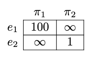
The maximin decision rule specifies that we should choose the policy that has the highest expected utility in the worst case environment. To evaluate which policy that is in this situation, for each policy, we identify the environment with the worst expected utility.

• Policy ${\pi }_1$ has either 100 utility (in $e_1$) or infinite utility (in $e_2$), so the worst case is 100 utility in environment $e_1$. 
•  Policy ${\pi }_2$ has either infinite (in $e_1$) utility or 1 utility (in $e_2$), so the worst case is 1 utility in environment $e_2$. 

Since ${\pi }_1$ has better worst case utility, we choose ${\pi }_1$, meaning we one box. The combination of the Nirvana Trick and the maximin decision rule allowed us to make the decision over the worlds that are logically possible. 

The IB agent achieves the desired behavior of one-boxing on Newcomb's problem. It also does this for the right reasons -- we are comparing the two logically possible situations and then picking the one with higher payoff, allowing us to make acausal considerations. 

Transparent Newcomb's Problem

Things get more tricky in the case that box B is transparent instead of opaque, meaning that you can see if Omega has put money into the box or not. We call this problem Transparent Newcomb's Problem. This problem is also discussed in the IB sequence [? · GW]. 

A full description of the game is: You have 2 transparent boxes (box A and box B) in front of you, and you have the option of taking either both boxes A and B (we call this 2-boxing), or taking just box B (we call this 1-boxing). Box A has $1 in it. A superintelligent agent, Omega, has put $100 in Box B if (and only if) it predicts that you would take only box B in the case that box B is full. 

Recall the decision rule above: ${\pi }^{\ast }={\text{argmax}}_{\pi \in \Pi }{\text{min}}_{e\in E}E(U;\pi ,e)$. Let's write out what each of these variables are in this context. 

The introduction of the new observable binary state means we double the number of policies, resulting in 4 possible policies:

• ${\pi }_{1,1}$ corresponds to 1-boxing in both cases 
• ${\pi }_{1,2}$ corresponds to 1-boxing if box B is empty and 2-boxing if box B is full
• ${\pi }_{2,1}$corresponds to 2-boxing if box B is empty and 1-boxing if box B is full
• ${\pi }_{2,2}$ corresponds to 2-boxing in both cases

I've enumerated them here, but the logic behind this notation is that the policy ${\pi }_{i,j}$ corresponds to  $i$-boxing if box B is empty and $j$-boxing if box B is full. The set of policies is $\Pi =\{{\pi }_{1,1},{\pi }_{1,2},{\pi }_{2,1},{\pi }_{2,2}\}$. 

Similarly, we have 4 environments, one associated with each policy. We denote the environments as $E=\{e_{1,1},e_{1,2},e_{2,1},e_{2,2}\}$. Each of these correspond to the environment in which, given Newcomb's problem, the agent uses the corresponding policy. For example, in the environment $e_{1,1}$ the agent is hardcoded to perform ${\pi }_{1,1}$, and so Omega, who has simulated the agent in this environment according to the hardcoded policy, will fill box B. (Meanwhile, our agent is living under Knightian uncertainty about which environment it is in, because it is still choosing which policy it will choose). 

So we have our set of actions, $\Pi$, and environments $E$ -- what's left is applying the Nirvana trick to our utility function $U$. Our utility is the dollar payoff of the chosen policy in the given environment, except in cases when our action given by the policy does not agree with the action given by the policy that is hardcoded in the environment. In these special cases, we apply the Nirvana Trick to give us infinite utility.  

All diagonal entries correspond to choosing the policy that matches the hardcoded policy, so these are simply the payoff in that situation. The Nirvana Trick applies whenever the agent chooses a policy that contradicts the environmental policy, AND we are in a branch of reality that the two disagree on. When we are in the environment $e_{1,1}$, Omega is predicting that we follow policy ${\pi }_{1,1}$, and so will fill box B with $100. If the agent chooses policy  ${\pi }_{2,1}$ (two box upon empty, one box upon full), since the box is indeed full, the action taken agrees with the action given by the hardcoded policy, and so we do not apply the Nirvana trick. On the other hand, we can send the policies ${\pi }_{1,2}$ and ${\pi }_{2,2}$ that do 2 box upon full, because in branch taken (box B is full), these policies contradict the hardcoded policy. 

Applying this reasoning over each environment-policy pair allows us to summarize the utility in the chart below. (Again this situation is deterministic, so the utility is the same as the expected utility.)

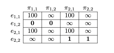
According to the IB decision rule, we should choose the action with the best worst case expected utility.  This means that: 

• ${\text{min}}_{e\in E}E(U;{\pi }_{1,1},e)={\text{min}}_{e\in E}E(U;{\pi }_{1,2},e)=0$
• ${\text{min}}_{e\in E}E(U;{\pi }_{2,1},e)={\text{min}}_{e\in E}E(U;{\pi }_{2,2},e)=1$

For ${\pi }_{1,1}$, the worst possible world is $e_{1,2}$, the world in which the hardcoded policy in the environment is ${\pi }_{1,2}$. In this world, reasons that you will act according to ${\pi }_{1,2}$ meaning that you would 2-box if Omega filled box B, and so Omega doesn't fill box B. However, ${\pi }_{1,1}$ and ${\pi }_{1,2}$ only give different actions when box B is full, and now that box B is empty, ${\pi }_{1,1}$ and${\pi }_{1,2}$ perform the same action -- 1-boxing. The action that the agent actually performs doesn't differ from the hardcoded policy, so we didn't send the agent to Nirvana. 

By 2-boxing in any case, you can always guarantee getting at least 1 utility, so the two optimal policies are the policies that 2-box in the case that box B is empty, which are ${\pi }_{2,1}$ and ${\pi }_{2,2}$.  

${\pi }_{2,2}$ is undesirable here because it ends up resulting in 1 utility, which is worse than the 100 utility that would be guaranteed by ${\pi }_{1,1}$ or ${\pi }_{1,2}$ . The reason for poor behavior is that the Nirvana trick is not forcing the hardcoded policy in the environment to match with the actual policy, instead, Nirvana is only forcing the hardcoded and actual policy to match in the branch that is actually taken.

The reason that IB fails here is that it violates the pseudo-causality condition, which says that the environment cannot depend on an agent's policy in a counterfactual that happens with probability 0. Transparent Newcomb's problem violates pseudo-causality. If you are an agent with the policy ${\pi }_{2,2}$, Omega punishes you by not filling up box B because if box B was full, you would 2-box. However, in this case, you never end up with a full box B, so this is the environment depending on an impossible world. 

One of the debates in Decision Theory overall is about what kind of scenarios are even fair to ask about. Eliezer argues in his TDT paper that one can always imagine a scenario that pays to everyone except those who follow a certain decision procedure, but of course these situations don't lend or take away credence to any decision scenario. A fairness condition should exclude these contrived scenarios, but other than that be as general as possible. The fairness condition for Infra-Bayesianism is the pseudo-causality condition, and if this holds, we have an optimality guarantee. 

Suppose we are given a decision scenario, like this one, that violates pseudo-causality. What can be done? There are two strategies that Vanessa highlights: 

1. Move the scenario into the pseudo-casual domain by introducing noise into the agent's action. We give the agent an $ϵ$ chance of exploring (taking a random action). This results in a policy that can get arbitrarily close to optimal. 
2. Extend the IB formalism to include infinitesimal probabilities. This works, but is hacky and makes the math much more convoluted. This is called using survironments and is addressed in this post [LW · GW]. 

Noisy Transparent Newcomb's problem 

The pseudo-causality condition only fails when we are certain that Omega will make the correct prediction. Suppose that Omega has an $ϵ$ chance of making the wrong prediction. Then, all outcomes happen with positive probability. From Murphy's perspective, whenever the hardcoded policy differs from the hardcoded policy in the environment, there is now always at least a slight chance of ending up in the situation where the agent actually realizes this difference, which would result in infinite utility, so Murphy is forced to choose the environment in which the hardcoded policy matches the agent's actual policy, in order to be sure that there is no chance of reaching Nirvana. This moves us back into the pseudo-causal domain, and results in IB achieving optimal behavior. 

For example, suppose that ${\pi }_{2,1}$ and $e_{1,1}$ are selected. ${\pi }_{2,1}$ means 2-boxing upon seeing empty and 1-boxing upon seeing full. The action hardcoded into the environment $e_{1,1}$ is ${\pi }_{1,1}$ (always 1 box), and because of this environment, Omega will fill up box B with probability $1-ϵ$, and in this case, the agent will see that box B is full, and so the agent will 1-box. However, there is an $ϵ$ probability that Omega will not fill up box B. In this case, the policy implemented by the agent (${\pi }_{2,1}$) tells it to 2-box, which differs with the hardcoded policy in the environment of always 1-boxing. Now that the action taken differs from the hardcoded policy, the utility goes to infinity, as specified by the Nirvana trick. Written out, the total expected utility is dominated by the small chance of Nirvana, meaning that Murphy will avoid this environment.  

$$E(U;{\pi }_{2,1},e_{1,1})=100(1-ϵ)+\infty \left(ϵ\right)=\infty$$

Similar reasoning across each policy environment pair results in the following expected utilities:

All of the off-diagonal entries are infinity, which leads to wonderful behavior -- the hardcoded policy in the environment is forced to match with the chosen policy. For each action, Murphy selects the environment that corresponds to that policy in order to avoid the infinite reward associated with Nirvana. Because of this, IB gives us the expected UDT behavior.  Assuming $ϵ\le .01$, the optimal policy is therefore ${\pi }_{2,1}$, as desired. 

The failure in transparent Newcomb's problem was because we were making our decision based off of worlds that were not logically possible, in which the hardcoded policy in the world does not match the policy taken by the agent. The Nirvana Trick, which is supposed to prevent this, fails because not every branch of the policy was executed. When box B is empty, we don't get to see what the agent would have done upon seeing a full box B. When the hardcoded policy and the agent's policy differ only on the branch that is not taken by reality, we cannot send the agent to Nirvana, because the hardcoded and the agent's policy are the same on the branch that was actually realized. These are the situations that violate pseudo-causality. 

We fix this by adding noise, meaning that each branch of the universe gets taken with at least some small probability. Then, any time the agent's policy differs from the hardcoded policy, there is at least some chance of infinite utility, meaning that Murphy always sends us to the world in which our policy matches the hardcoded policy. 

Conclusion

This post summarized some of the key insights behind Infra-Bayesianism. These insights included:

• Using imprecise probability to handle the non-realizability problem. 
• Using the maximin decision rule to select which probability to use out of your set of probability distributions, combined with the Nirvana Trick to avoid logically impossible worlds. 
• Applying the maximin decision rule to Newcomb's problem and transparent Newcomb's problem, and using this to motivate the pseudo-causality fairness condition. 

I intend to write further posts that go more into detail about the different parts of Infra-Bayesianism. If there is anything here that is particularly confusing, let me know and I will go into more depth in the future. Posts that are currently in the works include: 

• A detailed explanation of how off-branch expected utility can ensure dynamic consistency and several examples of this, as well as introducing affine measures and signed affine measures. 
• How Infra-Bayesianism could contribute to solving AI Alignment, as well as an explanation of which parts of embedded agency Infra-Bayesianism solves, which parts it might give a useful frame for, and which parts it does not help with.  

This post benefited from feedback given by Steve Zekany, Ashwin Sreevatsa, Jojo Lee, and Danny Oh.

9 comments

Comments sorted by top scores.