Finding Backward Chaining Circuits in Transformers Trained on Tree Search

post by abhayesian, Jannik Brinkmann (jannik-brinkmann), Victor Levoso · 2024-05-28T05:29:46.777Z · LW · GW · 1 comments

This is a link post for https://arxiv.org/abs/2402.11917

Contents

  Motivation & The Task
  Backward Chaining with Deduction Heads
  Register Tokens & Path Merging 
  Final Heuristic
  Tuned Lens Visualization
  Takeaways & Limitations 
  Future work
  Acknowledgments
None
1 comment

This post is a summary of our paper A Mechanistic Analysis of a Transformer Trained on a Symbolic Multi-Step Reasoning Task (ACL 2024). While we wrote and released the paper a couple of months ago, we have done a bad job promoting it so far. As a result, we’re writing up a summary of our results here to reinvigorate interest in our work and hopefully find some collaborators for follow-up projects. If you’re interested in the results we describe in this post, please see the paper for more details.

TL;DR - We train transformer models to find the path from the root of a tree to a given leaf (given an edge list of the tree). We use standard techniques from mechanistic interpretability to figure out how our model performs this task.  We found circuits that involve backward chaining - the first layer attends to the goal and each successive layer attends to the parent of the output of the previous layer, thus allowing the model to climb up the tree one node at a time. However, this algorithm would only find the correct path in graphs where the distance from the starting node to the goal is less than or equal to the number of layers in the model.  To solve harder problem instances, the model performs a similar backward chaining procedure at insignificant tokens (which we call register tokens).  Random nodes are chosen to serve as subgoals and the model backward chains from all of them in parallel.  In the final layers of the model, information from the register tokens is merged into the model’s main backward chaining procedure, allowing it to deduce the correct path to the goal when the distance is greater than the number of layers. In summary, we find a parallelized backward chaining algorithm in our models that allows them to efficiently navigate towards goals in a tree graph.

Motivation & The Task

Many people here have conjectured about what kinds of mechanisms inside future superhuman systems might allow them to perform a wide range of tasks efficiently. John Wentworth coined the term general-purpose search [LW · GW] to group several hypothesized mechanisms that share a couple of core properties. Others have proposed projects around how to search [LW · GW] for [LW · GW] search [LW · GW] inside neural networks.

While general-purpose search is still relatively vague and undefined, we can study how language models perform simpler and better-understood versions of search. Graph search, the task of finding the shortest path between two nodes, has been the cornerstone of algorithmic research for decades, is among the first topics covered by virtually every CS course (BFS/DFS/Djikstra), and serves as the basis for planning algorithms in GOFAI systems. Our project revolves around understanding how transformer language models perform graph search at a mechanistic level.

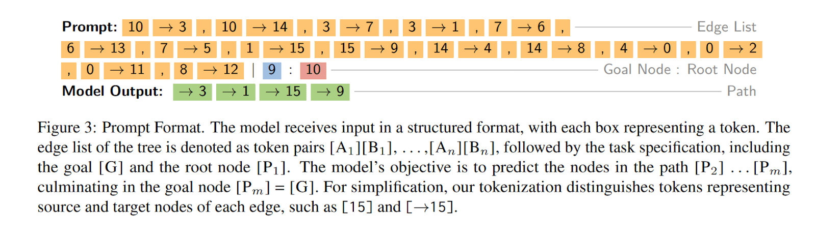
While we initially tried to understand how models find paths over any directed graph, we eventually restricted our focus specifically to trees. We trained a small GPT2-style transformer model (6 layers, 1 attention head per layer) to perform this task. The two figures below describe how we generate our dataset, and tokenize the examples.

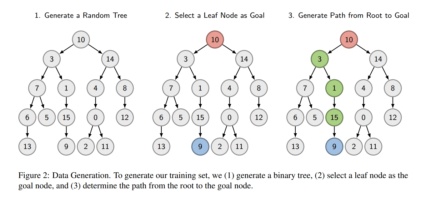
It is important to note that this task cannot be solved trivially. To correctly predict the next node in the path, the model must know the entire path ahead of time. The model must figure out the entire path in a single forward pass. This is not the case for a bunch of other tasks proposed in the literature on evaluating the reasoning capabilities of language models (see Saparov & He (2023) for instance). As a result of this difficulty, we can expect to find much more interesting mechanisms in our models.

We train our model on a dataset of 150,000 randomly generated trees. The model achieves an accuracy of 99.7 % on a test set of 15,000 unseen trees, despite seeing just a small fraction of all possible trees during training (the number of labeled binary trees is 16! times the 15th Catalan number, about 5.6 x 10¹⁹). This suggests that generalization is required for meaningful performance and that the model has learned to be capable of solving pathfinding in trees! 

 By analyzing the internal representations of the model, we identify several key mechanisms:

1. A specific type of copying operation is implemented in attention heads, which we call deduction heads. These are similar to induction heads as observed in Olsson et al. (2022). In our task, deduction heads intuitively serve the purpose of moving one level up the tree. These heads are implemented in multiple consecutive layers and allow the model to climb the tree multiple layers in a single inference step.
2. A parallelization motif whereby the early layers of the model choose to solve several subproblems in parallel that may be relevant for solving many harder instances of the task.
3. A heuristic that involves tracking the children of the current node and whether these children are leaf nodes of the tree. This mechanism is relevant when the model is unable to solve the problem using deduction heads in parallel.

Backward Chaining with Deduction Heads

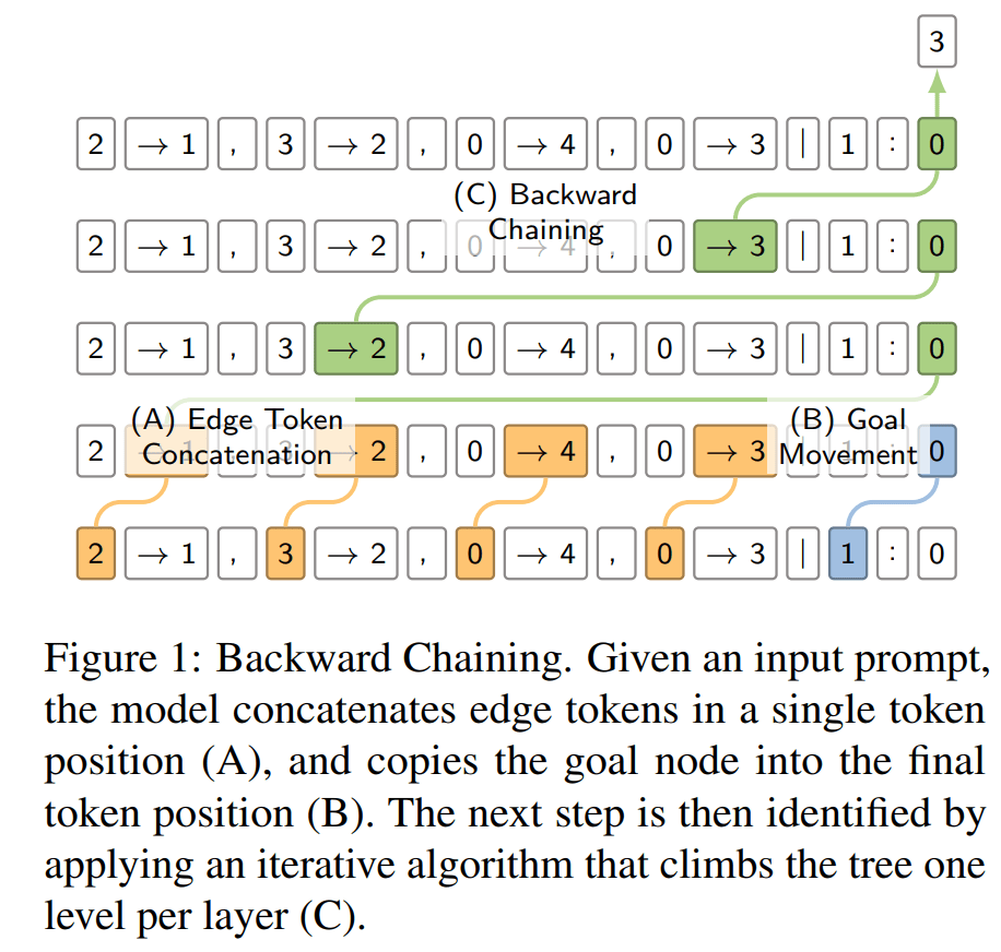
In this section, we describe the main backward chaining circuit. First, the model aggregates the source and target nodes of each edge in the edge list into the target node position. The model also moves information about the goal node into the last token position. Then, the model starts at the goal node and moves up the tree one level with each layer of the model. This process is depicted in the figure below.

The attention head in the first layer of the model creates edge embeddings by moving the information about the source token onto the target token for each edge in the context. Thus, for each edge [A][B] it copies the information from [A] into the residual stream at position [B]. This mechanism has some similarities with previous token heads, as observed in pre-trained language models (Olsson et al., 2022; Wang et al., 2023).

Another type of attention head involved in the backward chaining circuit is the deduction head. The function of deduction heads is to search for the edge in the context for which the current position is the target node [B], find the corresponding source token [A], and then copy the source token over to the current position. Thus, deduction heads complete the pattern by mapping: 

$$\text{[A] [B] ... [B] → [A]}$$

These heads are similar to the induction heads (which do [A] [B] ... [A] → [B]). The composition of a single previous token head and several deduction heads allows the model to form a backward chaining circuit. The attention heads of layers 2-6 can be partially described as deduction heads. This circuit allows the model to traverse the tree upwards for L − 1 edges, where L is the number of layers in the model.
 

  

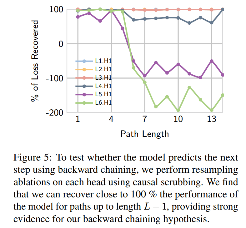
We provide several lines of evidence for backward chaining in our paper, involving a combination of visualizations, probing, and patching experiments. One particularly neat experiment from the paper is measuring how much of the model’s loss we can recover when we swap the output of an attention head with its activation on another input. According to our backward chaining hypothesis, the attention head of layer ℓ is responsible for writing the node that is ℓ − 1 edges above the goal into the final token position in the residual stream. This implies that the output of the attention head in layer ℓ should be consistent across trees that share the same node ℓ − 1 edges above the goal. If our hypothesized backward chaining circuit truly exists, then we should be able to generate two trees that share the same node ℓ − 1 edges above the goal node, substitute the output of the head (at the final token position) on one of the graphs with the output of the head on the other, and notice no change in the cross-entropy loss.

This procedure is similar to causal scrubbing [LW · GW] and allows us to measure the faithfulness of our hypothesis. In our experiment, we also separate examples by how far the root node is from the goal node in the clean graph (the graph we patch into, not the one we patch out of). The results of this experiment are presented in Figure 5 from our paper. For attention heads 1-4, we mostly notice no difference in the loss after performing the ablation. For attention heads 5 and 6, we mostly notice no difference in the loss after performing this ablation only if the goal is less than 5 edges from the current node. This means that most of the heads are doing backward chaining as we expected, but the last two layers of the model are doing something different only if the goal is further than L - 1 edges away. This discovery motivated our investigations in the following two sections of this post.

Register Tokens & Path Merging 

In the previous section, we showed that with the composition of multiple attention heads in consecutive layers, the model can traverse the tree upwards for L − 1 edges, where L is the number of layers in the model. However, this mechanism cannot explain the model’s performance in more complex scenarios, where the true path exceeds the depth of the mode. We find that the model does not only perform backward chaining on the final token position but in parallel at multiple different token positions, which we term register tokens. These subpaths are then merged on the final token position in the final two layers of the model.

The role of register tokens is to act as working memory. They are either tokens that do not contain any useful information, like the comma (“,”) or pipe (“|”) characters, or are tokens whose information has been copied to other positions, like the tokens corresponding to the source node of each edge. Register tokens are used to perform backward chaining from multiple subgoals in parallel before the actual goal is even presented in the context.

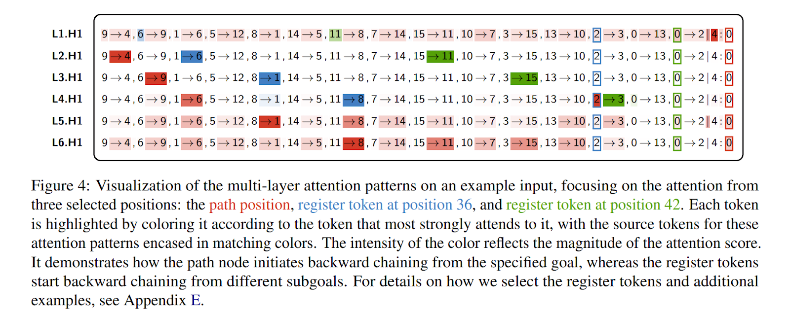
In the example above, you can see that two of the register token positions are backward chaining from specific subgoals in the same way that the final token position is backward chaining from the main goal. In the final 2-3 layers of the model, the final token position attends to the register tokens and moves the relevant information. We perform several additional experiments in our paper to verify that the register tokens are causally relevant to the model’s predictions. We also successfully train linear probes to extract information about subpaths from the residual steam at the register token positions.

Final Heuristic

There is an additional mechanism that helps the model avoid making illegal moves and hitting dead-ends. Attention heads L5.H1 and L6.H1 also promote the logits of children of the current node and suppress the logits of non-goal leaf nodes of the tree. When backward chaining and register tokens fail to find the full path, this heuristic allows the model to take a valid action and increases its probability of making its way onto the right path.

These two heads attend to the target node of every edge, except those for which the source node is the current path position. Remember that both nodes of the edge will be represented in the target node position. The output of these heads can be broken into three components:

1. Each edge decreases the logit of its target node.
2. Each edge increases the logit of its source node. 
3. Each token in the path decreases its logit.

As a result of these mechanisms, the logits of the leaf nodes in the graph will decrease while the logits of the children will increase. For the other nodes, the logit increase from being a parent and the logit decrease from being a child cancel each other out, causing their logit to remain the same. 

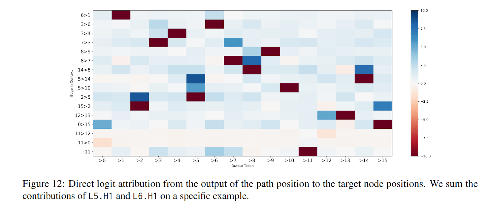
We can visualize this mechanism by looking at the sum of the contributions of L5.H1 and L6.H1 to the logits. We can visualize the exact contribution of each token in the context window to the logits through those two heads.

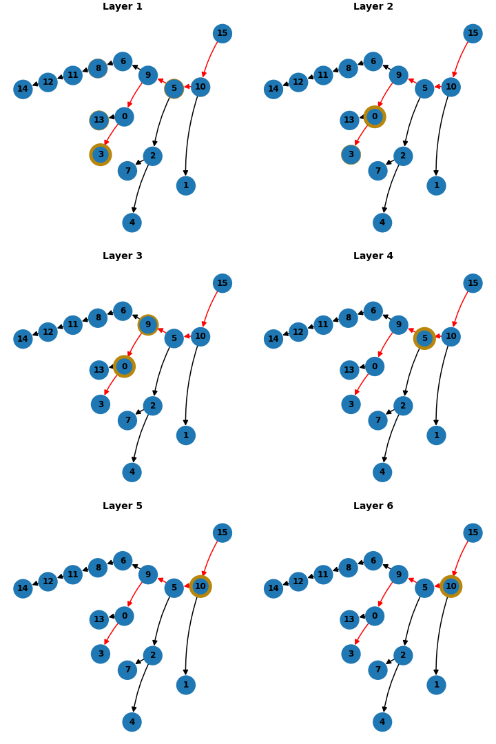
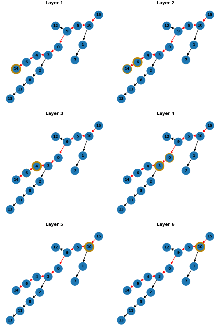
Tuned Lens Visualization

We use several different visualizations to demonstrate the backward chaining mechanisms. One of our favorites was inspired by the Tuned Lens (Belrose et al., 2023). We train a linear transformation to map residual stream activations after each layer to the final logits. We can project the estimated logits after each layer onto a tree structure, where the width of the yellow border is proportional to the magnitude of the probability.

 

   

 

Takeaways & Limitations 

Our work suggests that transformers may exhibit an inductive bias toward adopting highly parallelized search, planning, and reasoning strategies. Solving random subgoals at register tokens allows the model to get away with fewer serial computations than one might have naively assumed that it required to solve a problem. Transformers can waste parallel compute to make up for a deficit in serial compute.

One argument for why LLMs might learn to externalize their reasoning [LW · GW] by default is that the amount of planning they can do in a single forward pass is limited. They would need to write intermediate thoughts to a scratchpad so that they can progress in their planning/reasoning. However, they might also adopt a strategy similar to register tokens - they can implement a hidden scratchpad where they generate several sub-plans in parallel and merge the results in the final layers.

There are many limitations to our work:

1. All of our models only have a single head per layer. This bottleneck probably forces models to learn more interpretable mechanisms. 
2. When we trained our model, each edge list was randomly shuffled. However, we only interpret the models over the distribution of examples where the edges are ordered such that the source nodes are reverse topologically sorted. The model does something slightly different when the source nodes are topologically sorted because the causal mask forces the model to alternate strategies. Flipping the input allows the model to treat every target node token as a register token and the model backward chains from all 15 target node positions. This complexity hints at a core difficulty in mechanistic interpretability - it is hard to form simple hypotheses that explain the model’s performance over the entire training distribution.
3. We spent most of our time studying a single model. Other work has shown that the strong universality hypothesis is false; for example, different modular addition networks learn different algorithms (Zhong et al., 2023). We trained several other 6L1H models on this task and speculate that they probably learned something similar to register tokens by looking at their attention patterns, but not in the exact same way.
4. Trees are relatively simple compared to the broader class of directed graphs. We trained 6L4H models to successfully search for paths in directed graphs but had difficulties manually interpreting them due to the large number of components and their interactions.
5. There are broader questions about how useful these insights are for understanding actual language models. We discuss several similarities between mechanisms found in our models and mechanisms found in open-source large language models in our paper. There are also questions about whether mechanistic interpretability research reduces X-risk at all, but that’s a discussion for a different day [LW · GW].

Future work

Before working on this project, we worked on a related project that also involved using mechanistic interpretability on small models to understand planning and optimization in transformers.  We investigated whether models trained on setups similar to the one in Deepmind's In-context RL with Algorithm Distillation paper (Laskin et al., 2022) could learn to do RL in context or if they were just learning simpler heuristics instead.

That project was tabled while we worked on this one, but Victor is planning to continue working on it soon. Anyone interested in collaborating on this can go to the algorithm-distillation-project channel in the mechanistic interpretability discord server to express their interest.

We would also be interested in assisting other attempts to build off our work.

Acknowledgments

Jannik Brinkmann is supported by the German Federal Ministry for Digital and Transport (BMDV) and the German Federal Ministry for Economic Affairs and Climate Action (BMWK). 

Abhay Sheshadri and Victor Levoso have been supported by Lightspeed Grants.

Thanks to Erik Jenner and Mark Rybchuk for feedback.

 

1 comments

Comments sorted by top scores.