Crypto quant trading: Naive Bayes

post by Alexei · 2019-05-07T19:29:40.507Z · LW · GW · 13 comments

Contents

  What not to do
  One feature
  Using more recent data
  Additive smoothing
  Bet sizing
  Ignorant priors
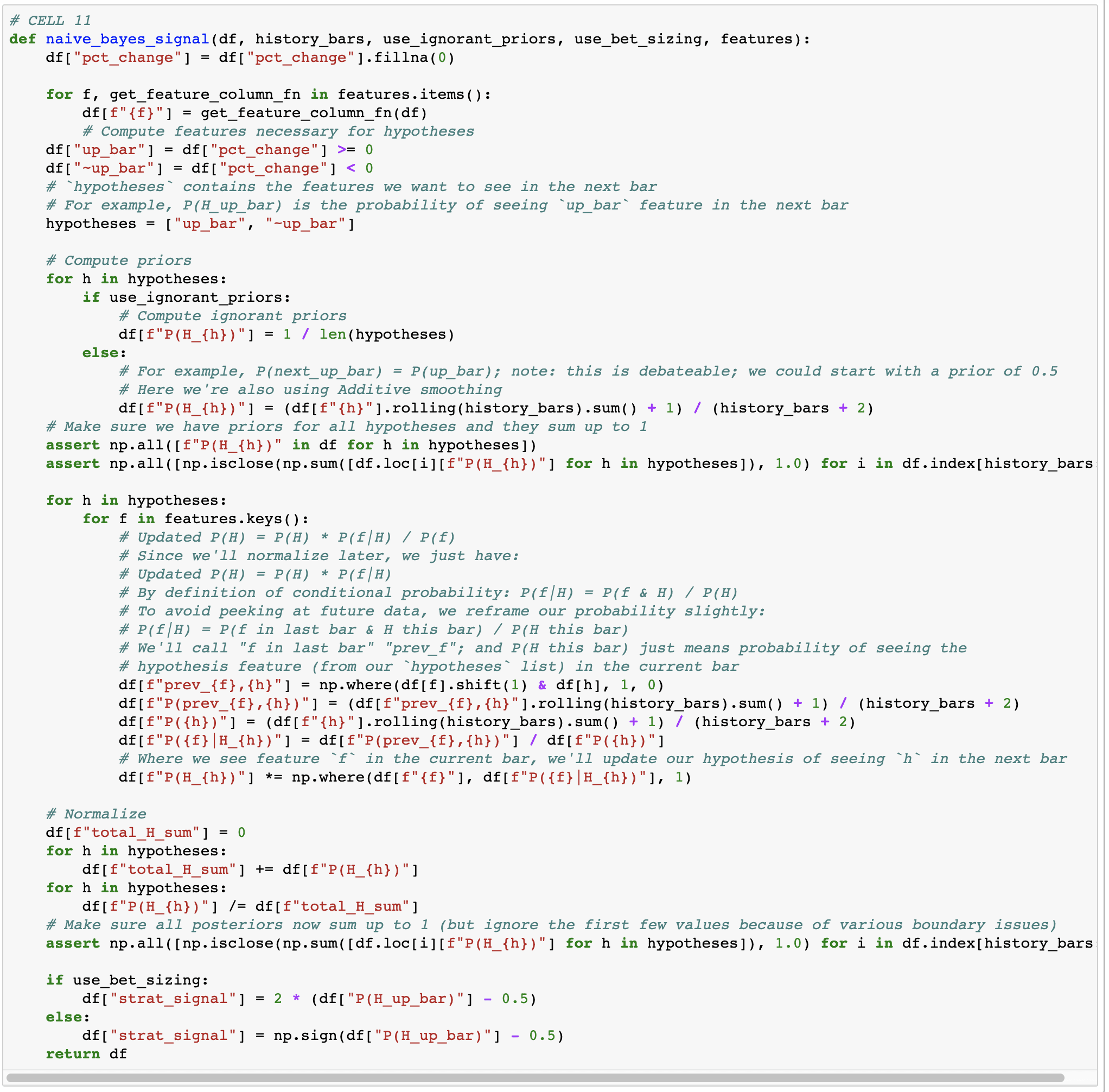
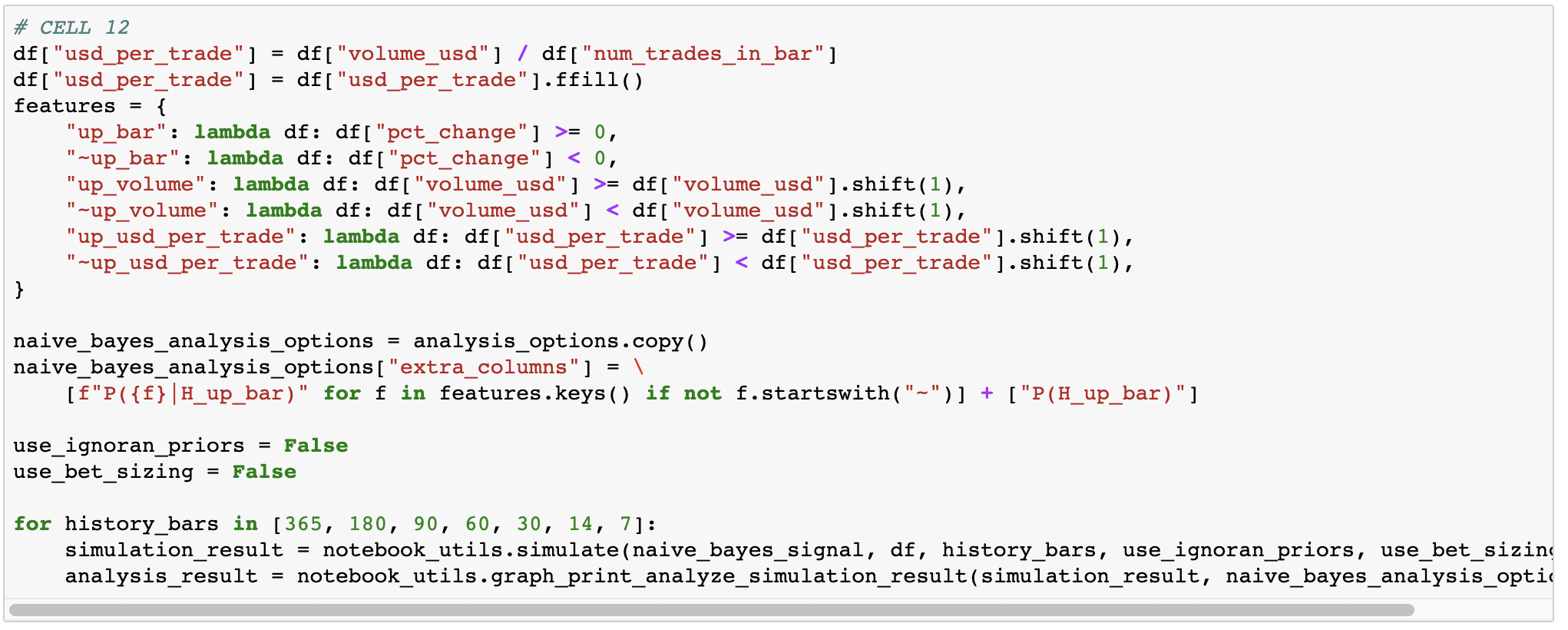
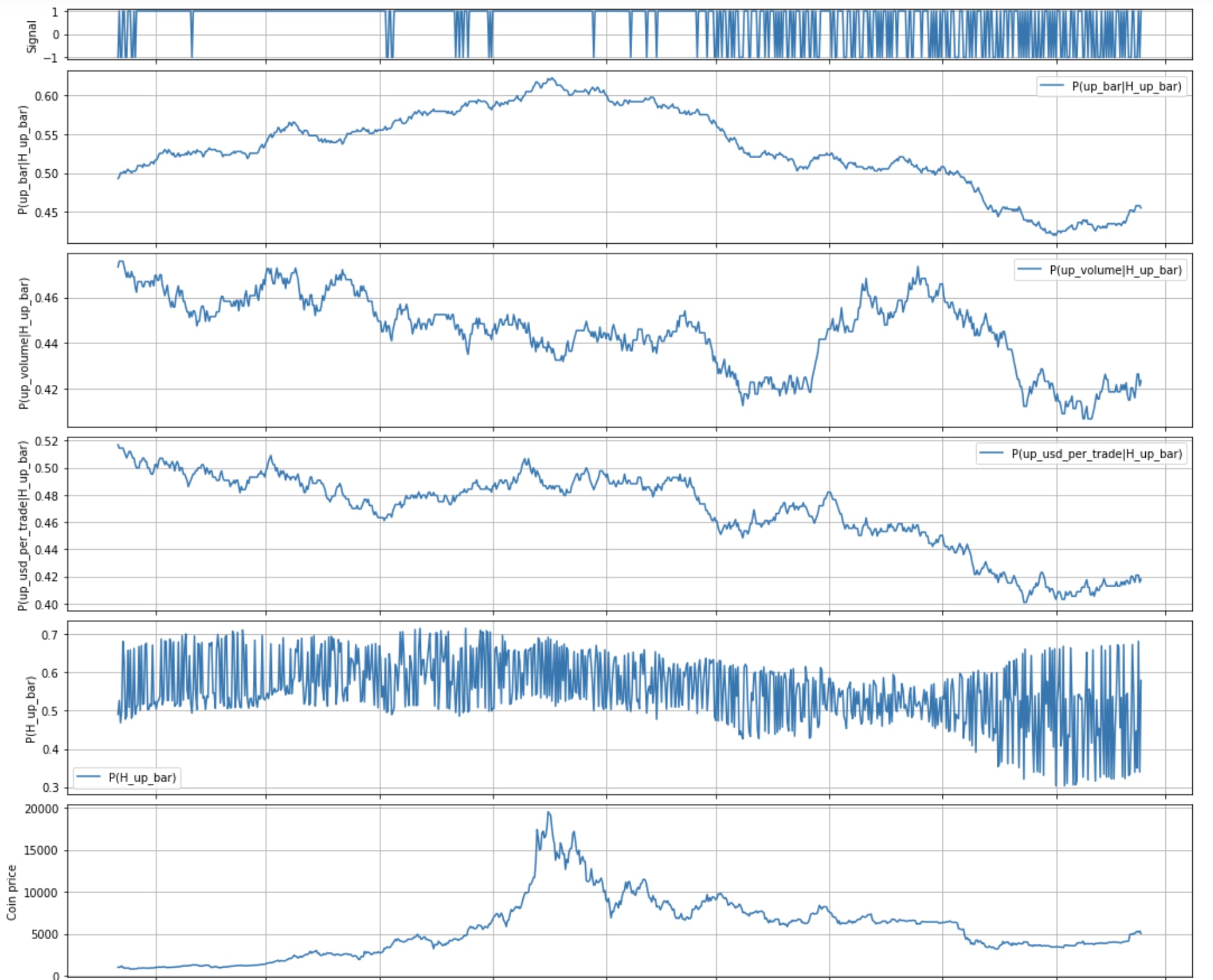
  Putting it all together with multiple features
  Homework
None
13 comments

Previous post: Crypto quant trading: Intro [LW · GW]

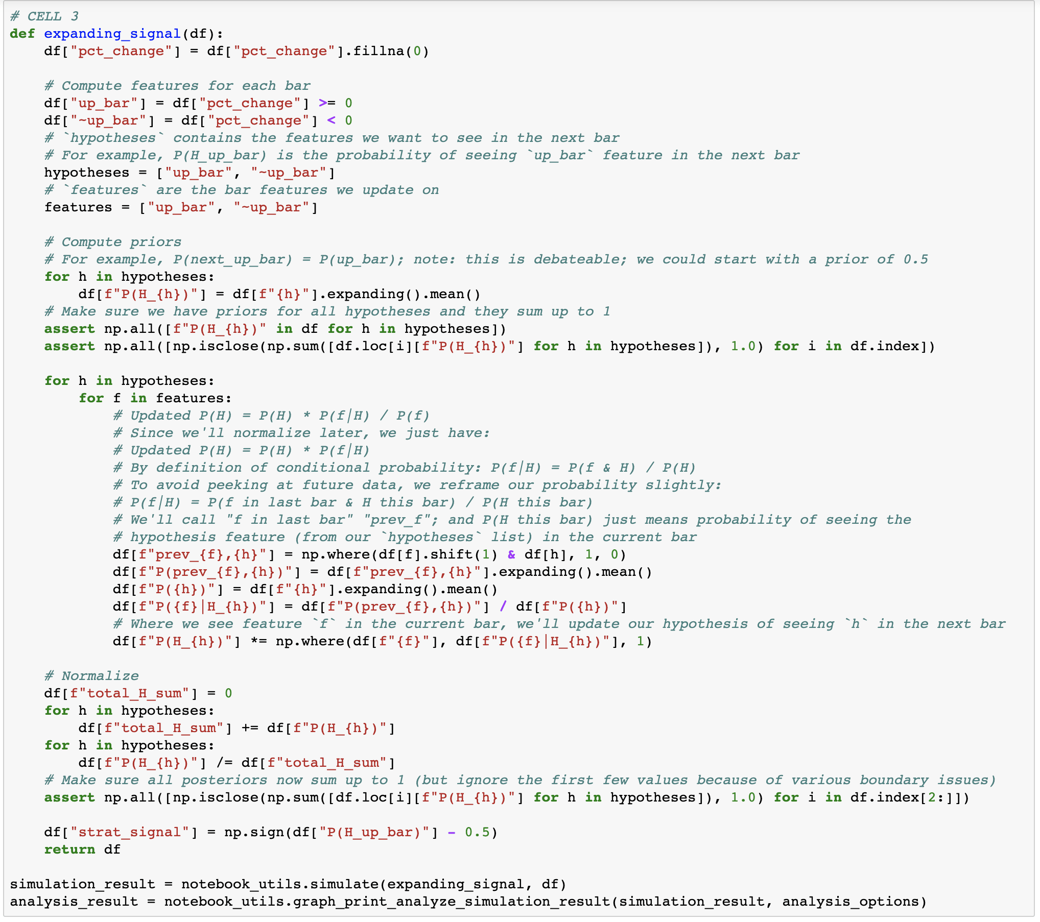
I didn't get requests for any specific subject from the last post, so I'm going in the direction that I find interesting and I hope the community will find interesting as well. Let's do Naive Bayes! You can download the code and follow along.

Just as a reminder, here's Bayes' theorem: P(H|f) = P(H) * P(f|H) / P(f). (I'm using f for "feature".)
Here's conditional probability: P(A|B) = P(A,B) / P(B)

Disclaimer: I was learning Naive Bayes as I was writing this post, so please double check the math. I'm not using 3rd party libraries so I can fully understand how it all works. In fact, I'll start by describing a thing that tripped me up for a bit.

What not to do

My original understanding was: Naive Bayes basically allows us to update on various features without concerning ourselves with how all of them interact with each other; we're just assuming they are independent. So we can just apply it iteratively like so:

P(H) = prior
P(H) = P(H) * P(f1|H) / P(f1)
P(H) = P(H) * P(f2|H) / P(f2)

You can see how that fails if we keep updating P(H) upwards over and over again, until it goes above 1. I did math the hard way to figure out where I went wrong. If we have two features:

P(H|f1,f2) = P(H,f1,f2) / P(f1,f2)
= P(f1|H,f2) * P(H,f2) / P(f1,f2)
= P(f1|H,f2) * P(f2|H) * P(H) / P(f1,f2)
= P(H) * P(f1|H,f2) * P(f2|H) / (P(f1|f2) * P(f2))
Then because we assume that all features are independent:
= P(H) * P(f1|H) * P(f2|H) / (P(f1) * P(f2))

Looks like what I wrote above. Where's the mistake? Well, Naive Bayes actually says that all features are independent, conditional on H. So P(f1|H,f2) = P(f1|H) because we're conditioning on H, but P(f1|f2) != P(f1) because there's no H in the condition.

One intuitive example of this is a spam filter. Let's say all spam emails (H = email is spam) have random words. So P(word1|word2,H)=P(word1|H), i.e. if we know email is spam, then the presence of any given word doesn't tell us anything about the probably of seeing another word. Whereas, P(word1|word2) != P(word1) since there are a lot of non-spam emails, where word appearances are very much correlated. (H/t to Satvik for this clarification.)

This is actually good news! Assuming P(f1|f2) = P(f1) for all features would be a pretty big assumption. But P(f1|H,f2) = P(f1|H), while often not exactly true, is a bit less of stretch and, in practice, works pretty well. (This is called conditional independence.)

Also, in practice, you actually don't have to compute the denominator anyway. What you want is the relative weight you should assign to all the hypotheses under consideration. And as long as they are mutually exclusive and collectively exhaustive, you can just normalize your probabilities at the end. So we end up with:

for each H in HS:
    P(H) = prior
    P(H) = P(H) * P(f1|H)
    P(H) = P(H) * P(f2|H)
    etc...
normalize all P(H)'s

Which is close to what we had originally, but less wrong.... Okay, now that we know what not to do, let's get on with the good stuff.

One feature

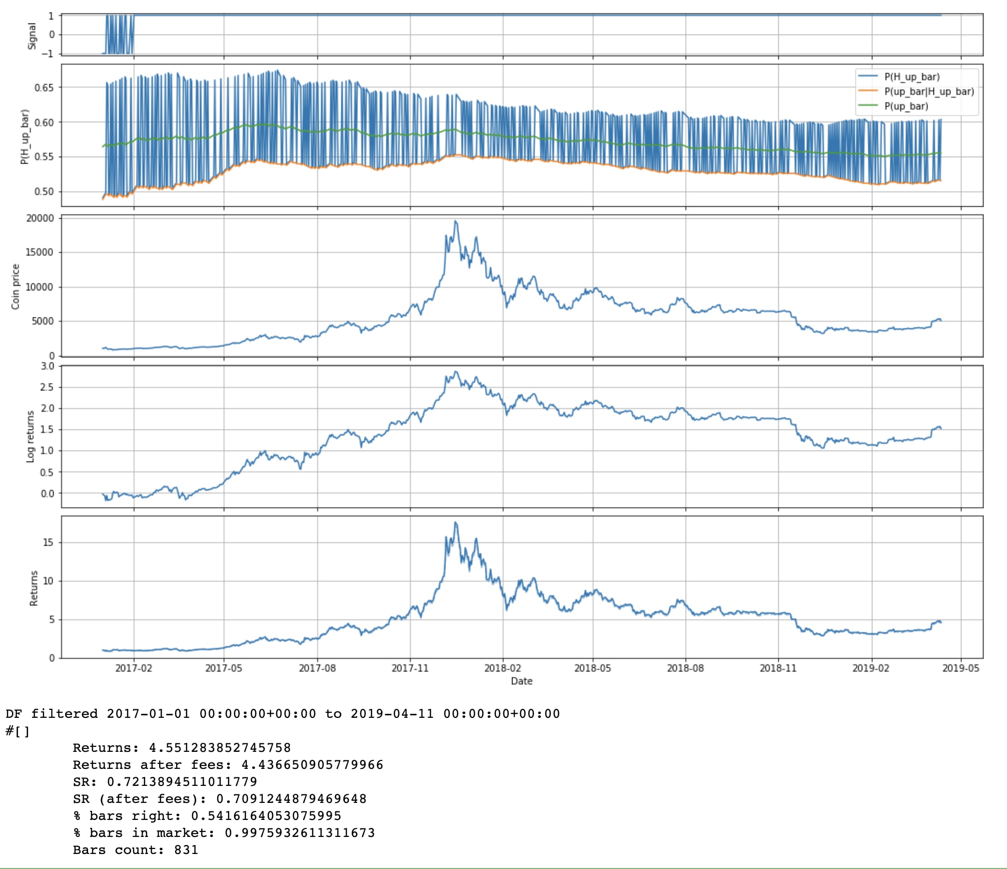
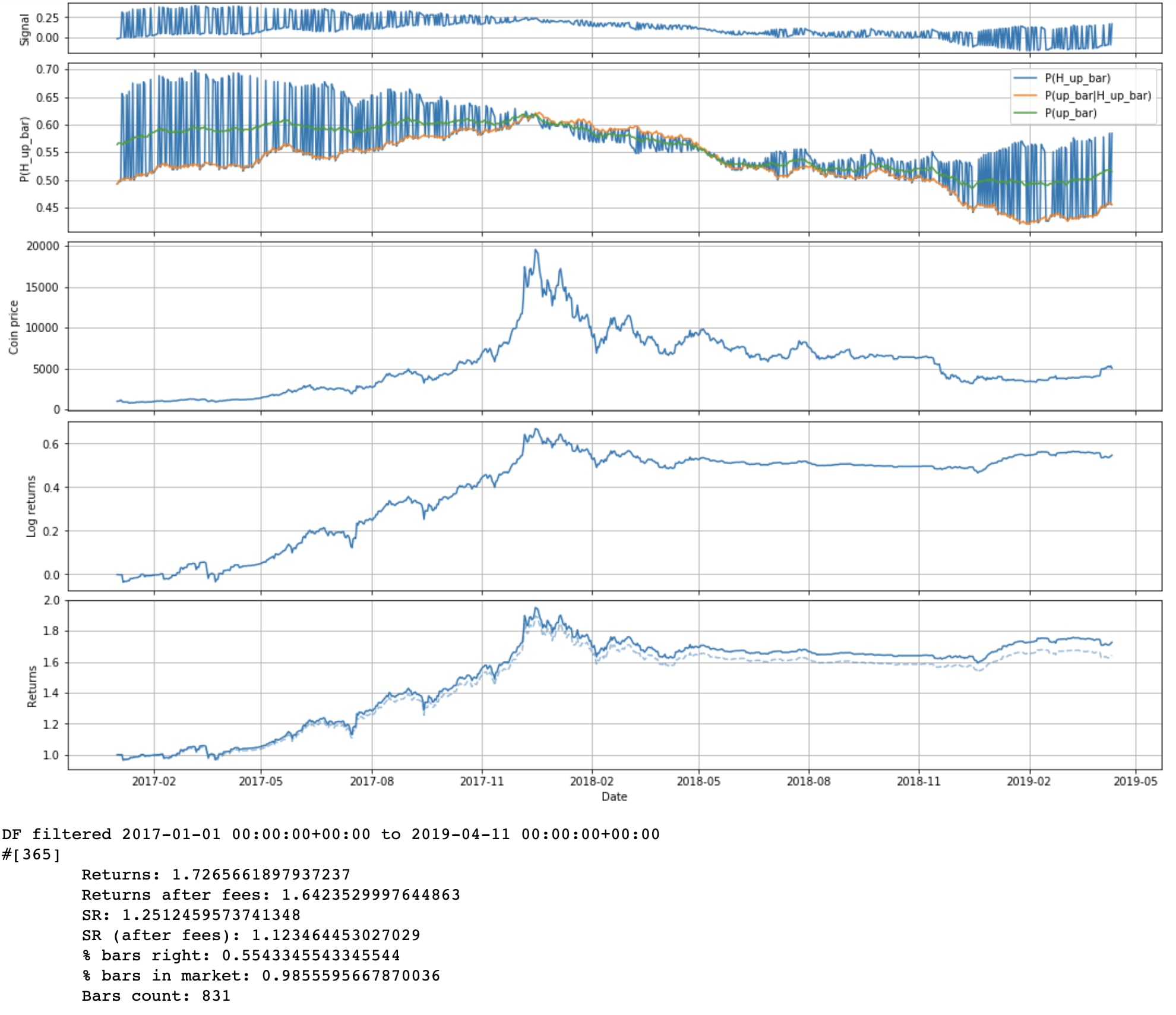
For now let's consider one very straight forward hypothesis: the closing price of the next day will be higher than today's (as a shorthand, we'll call tomorrow's bar an "up bar" if that's the case). And let's consider one very simple feature: was the current day's bar up or down?

Note that even though we're graphing only 2017 onwards, we're updating on all the data prior to that too. Since 2016 and 2017 have been so bullish, we've basically learned to expect up bars under either condition. I guess HODLers were right after all.

Using more recent data

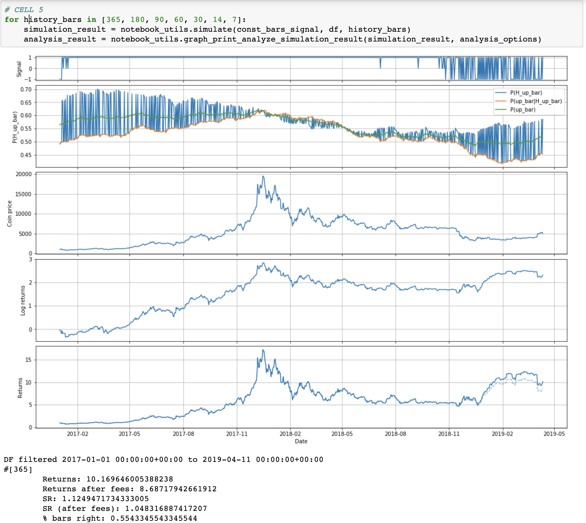
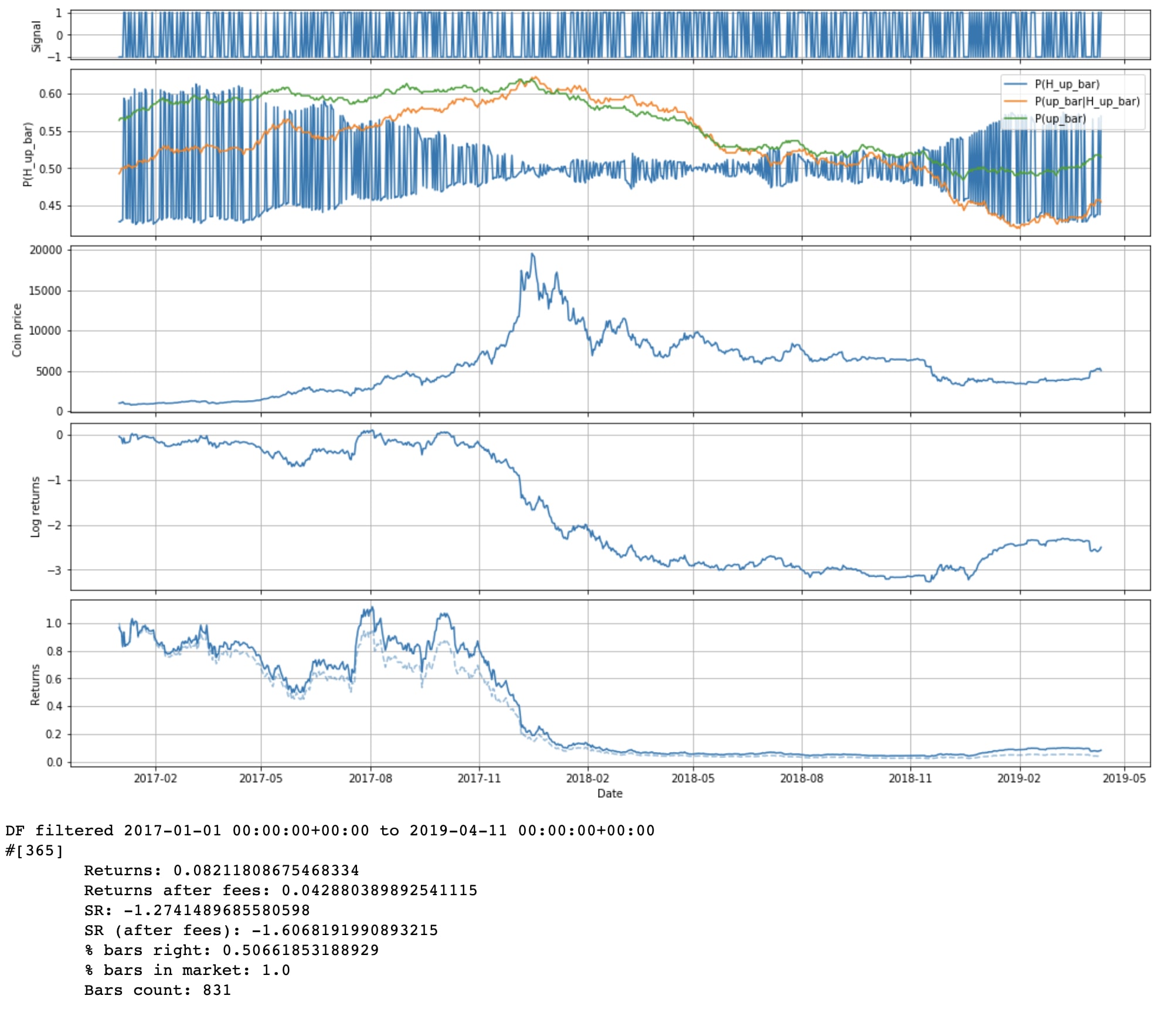
So, this approach is a bit suboptimal if we want to try to catch short term moves (like entire 2018). Instead, let's try to look at most recent data. (Question: does anyone know of Bayes-like method that weighs recent data more?)

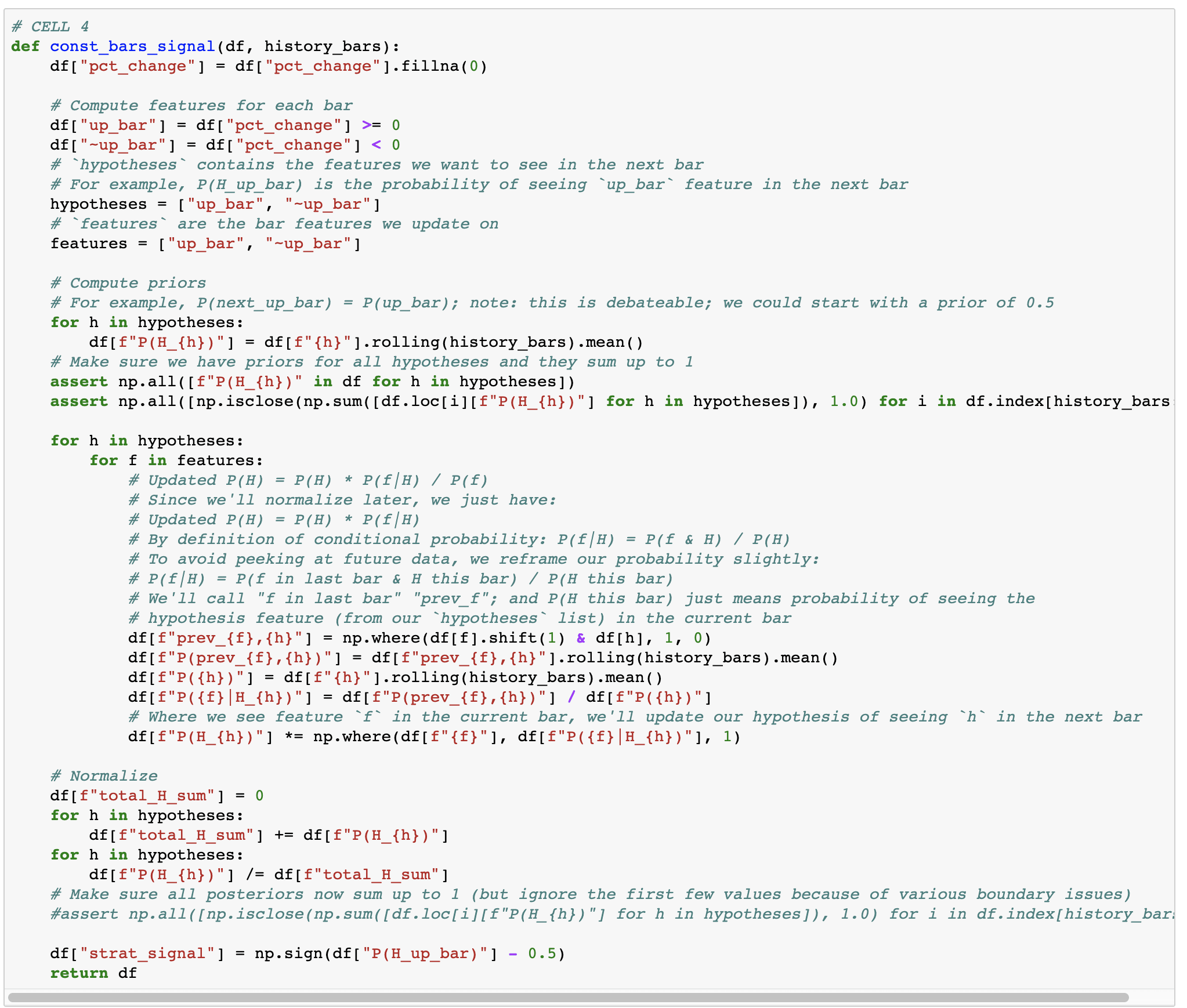
We slightly modify our algorithm to only look at and update on the past N days of data.

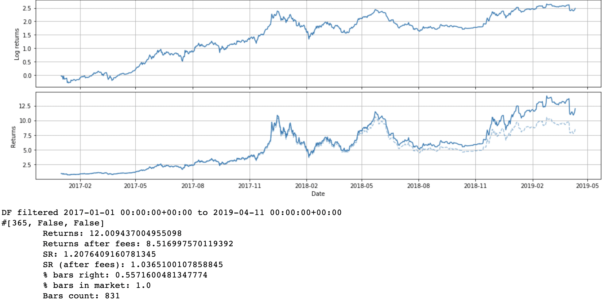
It's interesting to see that it still takes a while for the algorithm to catch up to the fact that the bull market is over. Just in time to not totally get crushed by the November 2018 drop.
In the notebook I'm also looking at shorter terms. There are some interesting results there, but I'm not going to post all the pictures here, since that would take too long.

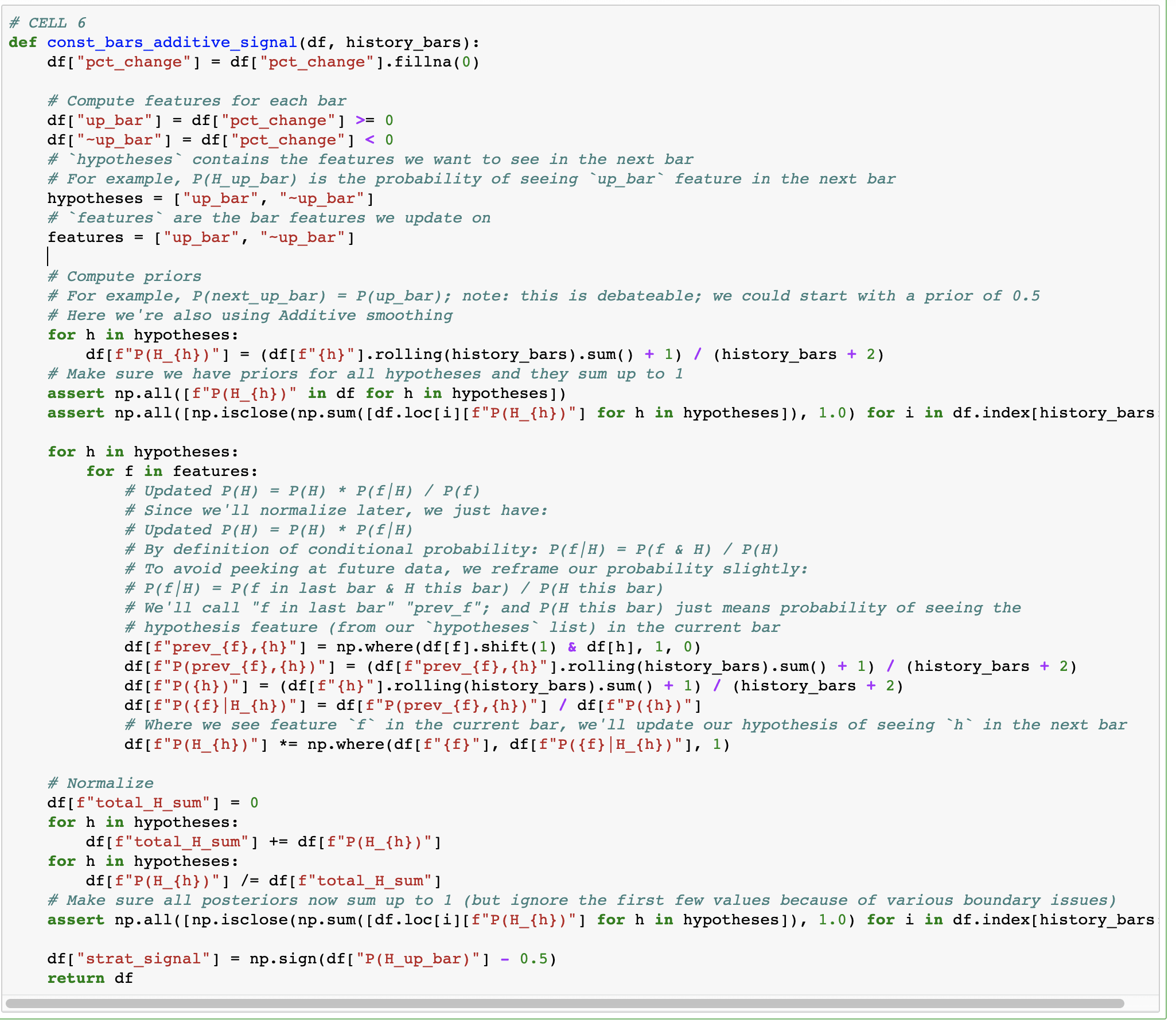
Additive smoothing

As we look at shorter and shorter timeframes, we are increasingly likely to run into a timeframe where there are only up bars (or only down bars) in our history. Then P(up)=1, which doesn't allow us to update [LW · GW]. (Some conditional probabilities get messed up too.) That's why we had to disable the posterior assert in the last code cell. Currently we just don't trade during those times, but we could instead assume that we've always seen at least one up and one down bar. (And, likewise, for all features.)

The results are not different for longer timeframes (as we'd expect), and mostly the same for shorter timeframes. We can reenable our posterior assert too.

Bet sizing

Currently we're betting our entire portfolio each bar. But in theory, our bet should probably be proportional to how confident we are. You could in theory use Kelly criterion, but you'd need to have an estimate of the size of the next bar. So for now we'll just try linear scaling: df["strat_signal"] = 2 * (df["P(H_up_bar)"] - 0.5)

We get lower returns, but slightly higher SR.

Ignorant priors

Currently we're computing the prior for P(next bar is up) by assuming that it'll essentially draw from the same distribution as the last N bars. We could also say that we just don't know! The market is really clever, and on priors we just shouldn't assume we know anything: P(next bar is up) = 50%.

# Compute ignorant priors
    for h in hypotheses:
        df[f"P(H_{h})"] = 1 / len(hypotheses)

Wow, that does significantly worse. I guess our priors are pretty good.

Putting it all together with multiple features

Homework

• Examine current features? Are they helpful / do they work?
• We're predicting up bars, but what we ultimately want is returns. What assumptions are we making? What should we consider instead?
• Figure out other features to try.
• Figure out other creative ways to use Naive Bayes.

13 comments

Comments sorted by top scores.