Calculating Natural Latents via Resampling

post by johnswentworth, David Lorell · 2024-06-06T00:37:42.127Z · LW · GW · 4 comments

Contents

  Some Conceptual Foundations
    What Are We Even Computing?
    Why Do We Want That, Again?
    Approximate “Uniqueness” and Competitive Optimality
  Strong Redundancy
  The Resampling Construction
    Theorem 1: Strong Redundancy => Naturality
    Theorem 2: Competitive Optimality
      Step 1: Xi Mediates Between Xj and X′i
      Step 2: X′ has Weak Redundancy over X
      Step 3: Λ Mediates between X and X′
      Step 4: Strong Redundancy of X′
    Can You Do Better?
  Empirical Results (Spot Check)
None
4 comments

So you’ve read some of our previous [LW · GW] natural latents [LW · GW] posts [LW · GW], and you’re sold on the value proposition. But there’s some big foundational questions still unanswered. For example: how do we find these natural latents in some model, if we don’t know in advance what they are? Examples in previous posts conceptually involved picking some latent out of the ether (like e.g. the bias of a die), and then verifying the naturality of that latent.

This post is about one way to calculate natural latents, in principle, when we don’t already know what they are. The basic idea is to resample all the variables once simultaneously, conditional on the others, like a step in an MCMC algorithm. The resampled variables turn out to be a competitively optimal approximate natural latent over the original variables (as we’ll prove in the post). Toward the end, we’ll use this technique to calculate an approximate natural latent for a normal distribution, and quantify the approximations.

The proofs will use the graphical notation introduced in Some Rules For An Algebra Of Bayes Nets [LW · GW].

Some Conceptual Foundations

What Are We Even Computing?

First things first: what even is “a latent”, and what does it even mean to “calculate a natural latent”? If we had a function to “calculate natural latents”, what would its inputs be, and what would its outputs be?

The way we use the term, any conditional distribution

$(\lambda ,x\mapsto P[\Lambda =\lambda |X=x\left]\right)$

defines a “latent” variable $\Lambda$ over the “observables” $X$, given the distribution $P\left[X\right]$. Together $P\left[X\right]$ and $P\left[\Lambda |X\right]$ specify the full joint distribution $P[\Lambda ,X]$. We typically think of the latent variable as some unobservable-to-the-agent “generator” of the observables, but a latent can be defined by any extension of the distribution over $X$ to a distribution over $\Lambda$ and $X$.

Natural latents are latents which (approximately) satisfy some specific conditions, namely that the distribution $P[X,\Lambda ]$ (approximately) factors over these Bayes nets:

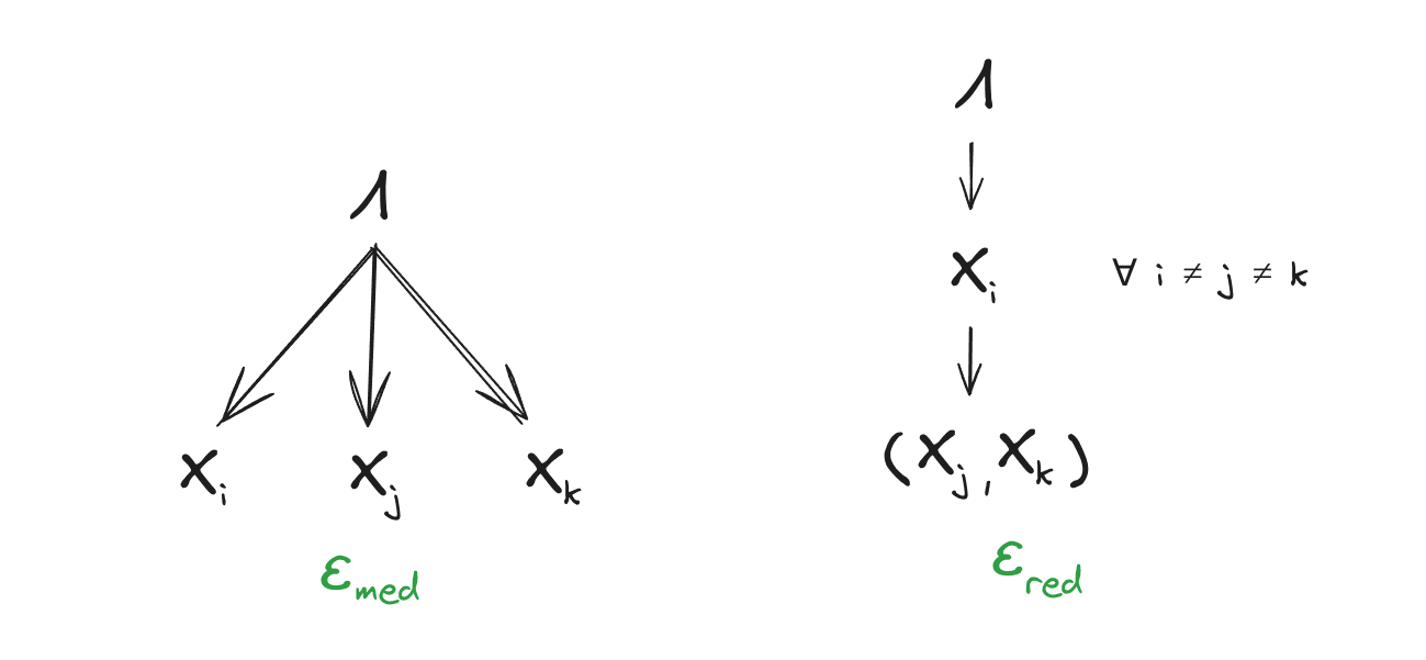
Intuitively, the first says that $\Lambda$ mediates between the $X_i$’s, and the second says that any one $X_i$ gives approximately the same information about $\Lambda$ as all of $X$. (This is a stronger redundancy condition than we used in previous posts; we’ll talk about that change below.)

So, a function which “calculates natural latents” takes in some representation of a distribution $(x\mapsto P[X\left]\right)$ over “observables”, and spits out some representation of a conditional distribution $(\lambda ,x\mapsto P[\Lambda =\lambda |X=x\left]\right)$, such that the joint distribution (approximately) factors over the Bayes nets above.

For example, in the last section of this post, we’ll compute a natural latent for a normal distribution. The function to compute that latent:

• Takes in a covariance matrix ${\Sigma }_{XX}$ for $X$, representing a zero-mean normal distribution $P\left[X\right]$.
• Spits out a covariance matrix ${\Sigma }_{\Lambda \Lambda }$ for $\Lambda$ and a cross-covariance matrix ${\Sigma }_{\Lambda X}$, together representing the conditional distribution of a latent $\Lambda$ which is jointly zero-mean normal with X.
• … and the joint normal distribution over $\Lambda ,X$ represented by those covariance matrices approximately factors according to the Bayes nets above.

Why Do We Want That, Again?

Our previous [LW · GW] posts [LW · GW] talk more about the motivation, but briefly: two different agents could use two different models with totally different internal (i.e. latent) variables to represent the same predictive distribution $P\left[X\right]$. Insofar as they both use natural latents, there’s a correspondence between their internal variables - two latents over the same $P\left[X\right]$ which both approximately satisfy the naturality conditions must contain approximately the same information about $X$. So, insofar as the two agents both use natural latents internally, we have reason to expect that the internal latents of one can be faithfully translated into the internal latents of the other - meaning that things like e.g. language (between two humans) or interpretability (of a net’s internals to a human) are fundamentally possible to do in a robust way. The internal latents of two such agents are not mutually alien or incomprehensible, insofar as they approximately satisfy naturality conditions and the two agents agree predictively.

Approximate “Uniqueness” and Competitive Optimality

There will typically be more than one different latent which approximately satisfies the naturality conditions (i.e. more than one conditional distribution $(\lambda ,x\mapsto P[\Lambda =\lambda |X=x\left]\right)$ such that the joint distribution of $\Lambda$ and $X$ approximately factors over the Bayes nets in the previous section). They all “contain approximately the same information about $X$”, in the sense that any one approximate natural latent approximately mediates between $X$ and any other approximate natural latent. In that sense, we can approximately talk as though the natural latent is unique, for many purposes. But that still leaves room for better or worse approximations.

When calculating, we’d ideally like to find a natural latent which is a “best possible approximate natural latent” in some sense. Really we want a pareto-best approximation, since we want to achieve the best approximation we can on each of the naturality conditions, and those approximations can trade off against each other.

… but there’s a whole pareto surface, and it’s a pain to get an actual pareto optimum. So instead, we’ll settle for the next best thing: a competitively optimal approximate natural latent. Competitive optimality means that the natural latent we’ll calculate approximates the naturality conditions to within some bounds of any pareto-best approximate natural latent; it can only do so much worse than “the best”. Crucially, competitive optimality means that when we don’t find a very good approximate natural latent, we can rule out the possibility of some better approximate natural latent.

Strong Redundancy

Our previous posts on natural latents used a relatively weak redundancy condition: all-but-one $X_i$ gives approximately the same information about $\Lambda$ as all of $X$. (Example: 999 rolls of a biased die give approximately the same information about the bias as 1000 rolls.) The upside of this condition is that it’s relatively general; the downside is that it gives pretty weak quantitative bounds, and in practice we’ve found that a stronger redundancy condition is usually more useful. So in this post, we’ll require “strong redundancy”: any one $X_i$ must give approximately the same information about $\Lambda$ as all of $X$. (Example: sticking a thermometer into any one part of a bucket of water at equilibrium gives the same information about the water’s temperature.)

If we want to turn weak redundancy into strong redundancy, e.g. to apply the methods of this post to the biased die example, the usual trick is to chunk together the $X_i$’s into two or three chunks. For instance, with 1000 die rolls, we could chunk together the first 500 and the second 500, and either of those two subsets gives us roughly the same information about the bias (insofar as 500 rolls is enough to get a reasonably-precise estimate of the bias).

Conceptually, with strong redundancy, all of the $X$-relevant information in a natural latent is represented in every single one of the $X_i$’s. For purposes of establishing that e.g. natural latents of two different agents contain the same information about $X$, that means strong redundancy gives us “way more than we need” - we only really need strong redundancy over two or three variables in order to establish that the latents “match”.

The Resampling Construction

We start with a distribution $P\left[X\right]$ over the variables $X_1\dots X_n$. We want to construct a latent which is competitively optimal - i.e. if any latent exists over $X_1\dots X_n$ which satisfies the natural latent conditions to within some approximation, then our latent satisfies the natural latent conditions to within some boundedly-worse approximation (with reasonable bounds). We will call our competitively optimal latent $X^{\prime }$ (pronounced “X prime”), for reasons which will hopefully become clear shortly.

Here’s how we construct $X^{\prime }$. Take “X”, then add an apostrophe, “‘“, like so -> X’ … and that was how David died. Anyway, to construct $X^{\prime }$:

• For each $i$, obtain $X_i^{\prime }$ by sampling from the distribution of $X_i$ given all the other $X_j$’s.
• Stack those up to obtain $X^{\prime }$.

Mathematically, that means the defining distribution of the latent $X^{\prime }$ is

$P[X^{\prime }=x^{\prime }|X=x]={\prod }_{i}P[X_i=x_i^{\prime }|X_{\overline{i}}=x_{\overline{i}}]$

Conceptually, we can think of this as a single resample step of the sort one might use for MCMC, in which we resample every variable simultaneously conditional on all other variables.

Example: suppose $X_1$ is 500 rolls of a biased die, $X_2$ is another 500 rolls of the same die, and $X_3$ is yet another 500 rolls of the same die. Then to calculate $X_1^{\prime }$. I sample the bias of the die conditional on the 1000 rolls in $X_2$ and $X_3$, then generate 500 new rolls of a die with my newly-sampled bias, and those new rolls are $X_1^{\prime }$. Likewise for $X_2^{\prime }$ and $X_3^{\prime }$ (noting that I’ll need to sample a new bias for each of them). Then, I put all those 1500 rolls together to get $X^{\prime }$.

Why would $X^{\prime }$ be a competitively optimal natural latent? Intuitively, if there exists a natural latent (with strong redundancy), then each $X_i$ encodes the value of the natural latent (approximately) as well as some “noise” independent of all the other $X_i$’s. When we resample, the natural latent part is kept the same, but the noise is resampled to be independent of the other $X_i$’s. So, the only information which $X^{\prime }$ contains about $X$ is the value of the natural latent. Of course, that story doesn’t give approximation bounds; that’s what we’ll need all the fancy math for.

In the rest of this section, we’ll show that $X^{\prime }$ satisfies the naturality conditions competitively optimally: if there exists any latent $\Lambda$ which is natural to within some approximation, then $X^{\prime }$ is natural to within a boundedly-worse approximation.

Theorem 1: Strong Redundancy => Naturality

Normally, a latent must approximately satisfy two (sets of) conditions in order to be natural: mediation, and redundancy. The latent must encode approximately all the information correlating the $X_i$’s (mediation), and each $X_i$ must give approximately the same information about the latent (redundancy). Theorem 1 says that, for $X^{\prime }$ specifically, the approximation error on the (strong) redundancy conditions upper bounds the approximation error on the mediation condition. So, for $X^{\prime }$ specifically, “redundancy is all you need” in order to establish naturality.

Some of the proof will be graphical, but we’ll need to start with one key algebraic step. The key step is this:

$D_{KL}\left(P\right[X,X^{\prime }\left]||P\right[X^{\prime },X_j\left]P\right[X_{\overline{j}}|X_j\left]\right)=E\left[lnP\right[X_{\overline{j}}|X_j,X^{\prime }]-lnP[X_{\overline{j}}|X_j\left]\right]$

$=E\left[lnP\right[X_{\overline{j}}|X_j,X^{\prime }]-lnP[X_{\overline{j}}|X_j^{\prime }\left]\right]$

$=D_{KL}\left(P\right[X,X^{\prime }\left]||P\right[X^{\prime },X_j\left]P\right[X_{\overline{j}}|X_j^{\prime }\left]\right)$

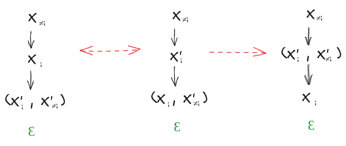
The magic piece is the replacement of $E\left[lnP\right[X_{\overline{j}}|X_j\left]\right]$ with $E\left[lnP\right[X_{\overline{j}}|X_j^{\prime }\left]\right]$; this is allowed because, by construction, $(X_{\overline{j}},X_j)$ have the exact same joint distribution as $(X_{\overline{j}},X_j^{\prime })$. Graphically, that tells us:

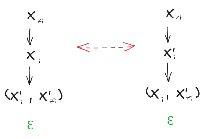
Note that the left diagram is the strong redundancy condition for $X_i$.

The rest of the proof is just a bookkeeping step:

So $X^{\prime }$ mediates between $X_i$ and $X_{\overline{i}}$, for all $i$.

Theorem 2: Competitive Optimality

To prove competitive optimality, we first assume that there exists some latent $\Lambda$ over $X$ which satisfies the (strong) natural latent conditions to within some bounds. Using that assumption, we want to prove that $X^{\prime }$ satisfies the (strong) natural latent conditions to within some not-much-worse bounds. And since Theorem 1 showed that, for $X^{\prime }$ specifically, the strong redundancy approximation error bounds the mediation approximation error, all that’s left is to bound the strong redundancy approximation error for $X^{\prime }$.

Outline:

• First, assuming a strong approximate natural latent $\Lambda$ exists, we’ll show that any $X_i$ approximately mediates between any other $X_j$, $X_k$. (This is a handy property in its own right!)
• Second, we’ll show that $X^{\prime }$ satisfies a weak redundancy condition over X.
• Third: since a natural latent is the “maximal” latent which satisfies redundancy over X [LW · GW], the previous condition is in-principle sufficient to show that $\Lambda$ approximately mediates between $X^{\prime }$ and $X$. However, we’ll inline the proof of the maximality condition and tweak it a bit to get slightly better bounds.
• Since we can sample $\Lambda$ equally well with any one $X_i$ (i.e. strong redundancy), and $\Lambda$ approximately tells us everything $X$ tells us about $X^{\prime }$, we can sample $X^{\prime }$ equally well with any one $X_i$: strong invariance holds for $X^{\prime }$.

Step 1: $X_i$ Mediates Between $X_j$ and $X_i^{\prime }$

The two naturality conditions (just one of the $N$ redundancy conditions) of $\Lambda$ over $X$ easily show that $X_i$ mediates between $X_j$ and $X_k$ ($i\ne j\ne k$). The equivalence of $P\left[X\right]$ and $P[X_i,X_j,X_k^{\prime }]$ (by construction of $X^{\prime }$) allows for replacing $X_k^{\prime }$ in the factorization with the $X_k^{\prime }$ version. Then, we get the result we were looking for.

Step 2: $X^{\prime }$ has Weak Redundancy over $X$

In the first line, we use the definition of $X^{\prime }$ and the result from Step 1 to establish mediation of $X_1$ between $X_2$ and $X_3^{\prime }$ and so we can remove the outgoing edge $X_2\to X_3^{\prime }$. In the second line, we do the same thing for the remaining outgoing edge of $X_2$, establishing $X_2$ as unconditionally independent of $X^{\prime }$. Having done so, $(X_1,X_3)$ trivially mediates between $X_2$ and $X^{\prime }$.

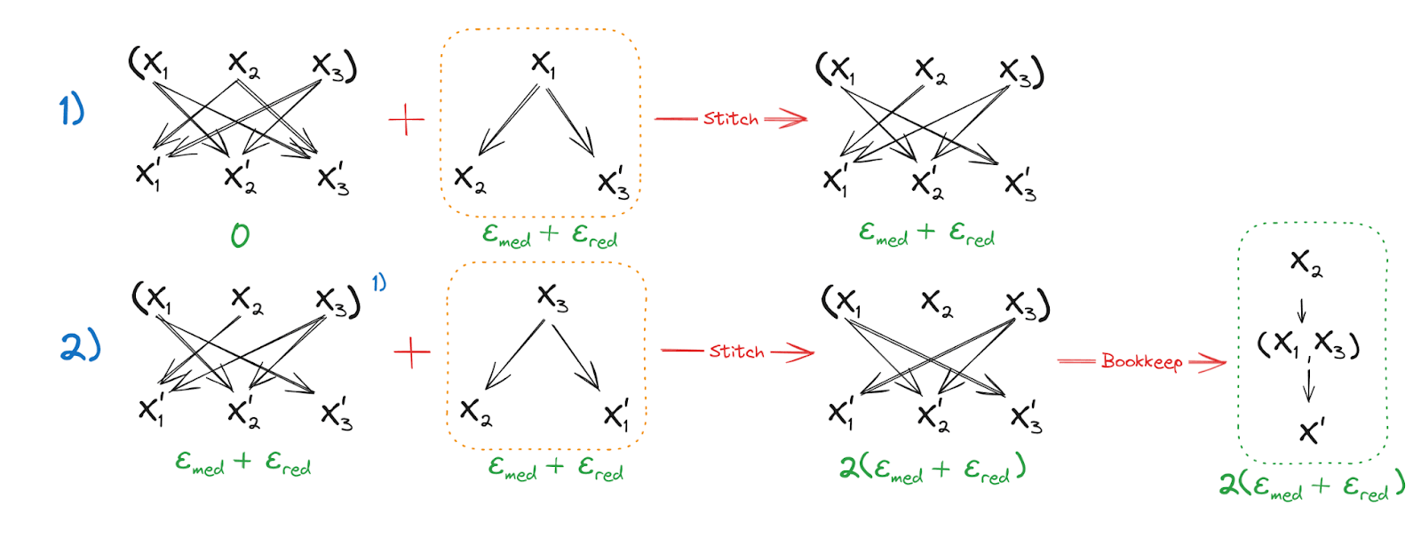
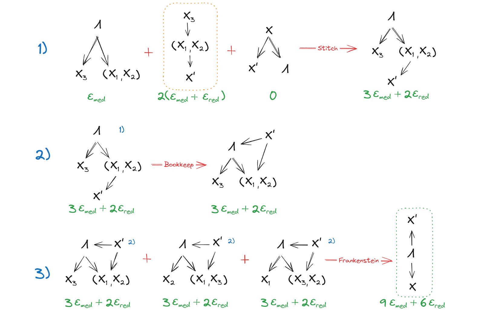
Step 3: $\Lambda$ Mediates between $X$ and $X^{\prime }$

The intermediates here are much more easily understood in graphical form, but in words: In lines 1 and 2, we combine result of Step 2 with the mediation condition of $\Lambda$ and the definition of $X^{\prime }$ to stitch together a combined factorization of the joint distribution of $X$, $X^{\prime }$, and $\Lambda$ where $X$ mediates between $\Lambda$ and $X^{\prime }$, and in particular it’s the components $(X_1,X_2)$ which mediate while $X_3$ is independent conditional on $\Lambda$. With some minor bookkeeping, we flip the arrow between $(X_1,X_2)$ and $X^{\prime }$, and add an arrow from $X^{\prime }$ to $\Lambda$. Since this produces no cycles nor colliders, this is a valid move.

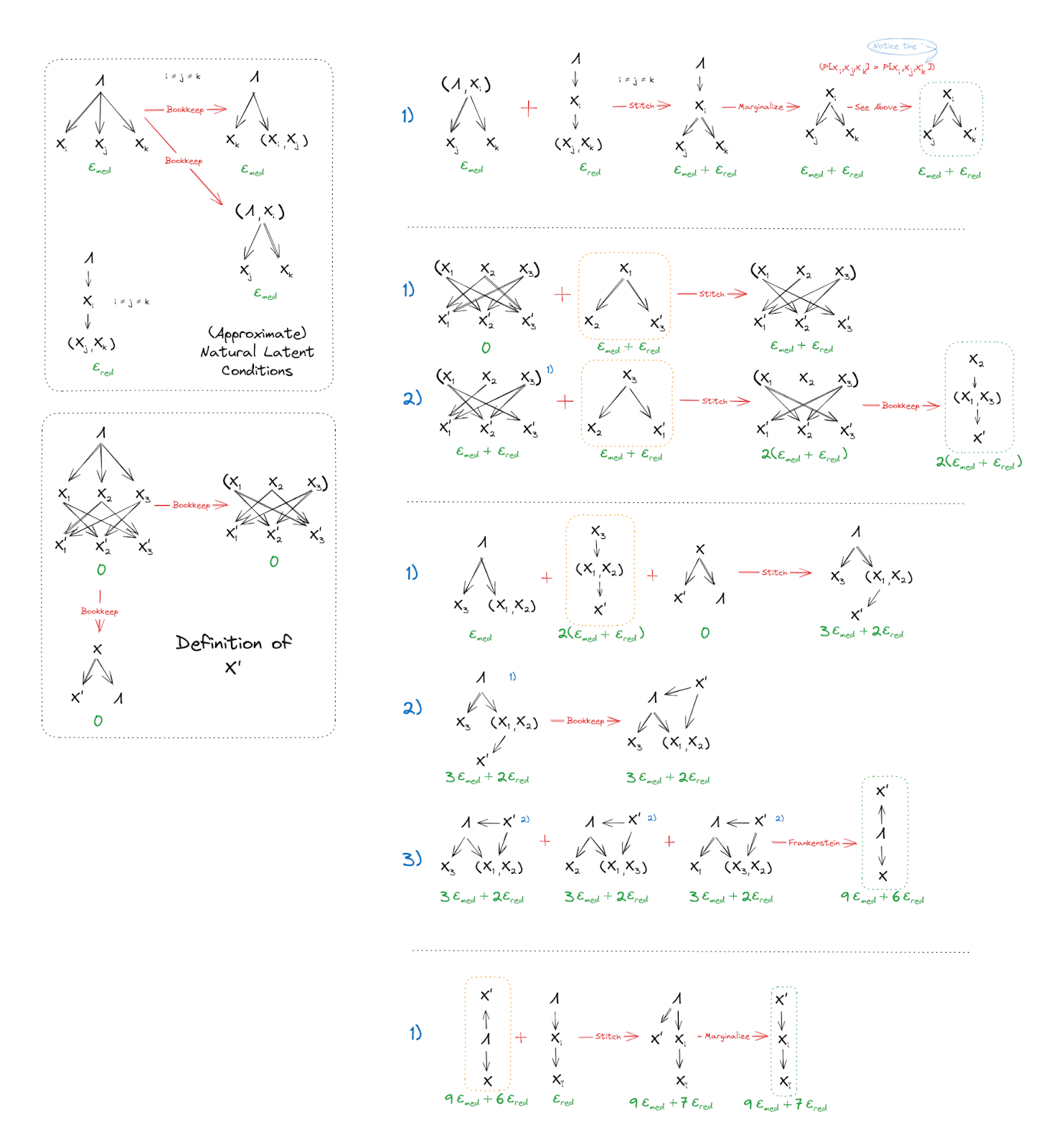
In line three, we use the result of line 2 in all 3 permutations of the $X$ components and Frankenstein the graphs together to show that, since each component of $X$ has $\Lambda$mediating between it and $X^{\prime }$, $\Lambda$ mediates between all of $X$ and $X^{\prime }$.

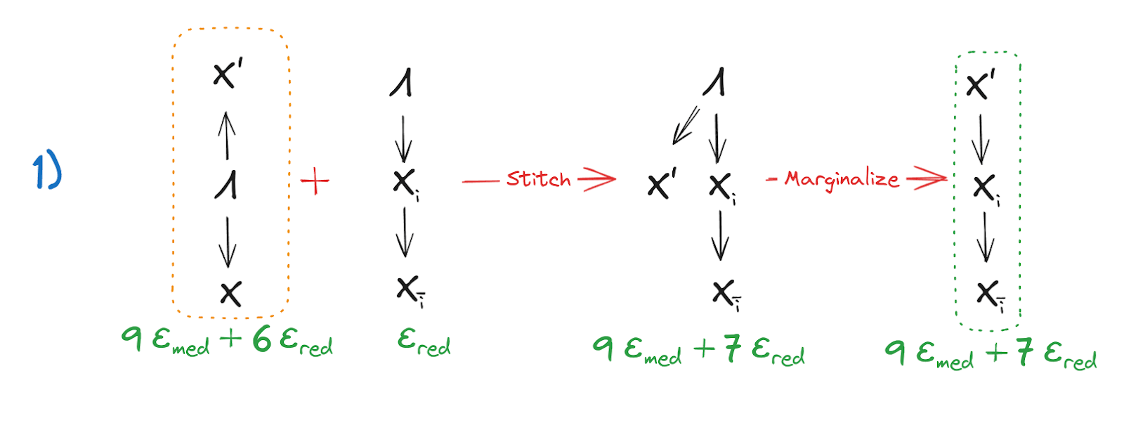
Step 4: Strong Redundancy of $X^{\prime }$

Using the result from Step 3, along with the strong redundancy of $\Lambda$ allows us to stitch the graphs together and finally obtain our desired result: Strong Redundancy of $X^{\prime }$. 

The full proof of (Approximate) Natural Latent => (Approximate) Strongly Redundant $X^{\prime }$ in one picture:

Can You Do Better?

Note that the bounds derived here are fine in a big-O sense, but a little… unaesthetic. The numbers 9 and 7 are notably not, like, 1 or 2 or even 3. Also, we had to assume a strong approximate natural latent over at least three variables in order for the proof to work; the proof actually doesn’t handle the 2-variable case!

Could we do better? In particular, a proof which works for two variables would likely improve on the bounds considerably. We haven’t figured out how to do that yet, but we haven’t spent that much time on it, and intuitively it seems like it should work.

So if you’re good at this sort of thing, please do improve on our proof!

Empirical Results (Spot Check)

As an empirical check, we coded up relevant calculations for normal distributions. We are not going to go through all the linear algebra in this post, but you can see the code here, if for some reason you want to inflict that upon yourself. The main pieces are:

• Methods to calculate covariance matrices for various conditionals and marginals
• A method to construct the joint covariance of $X$ and $X^{\prime }$
• A method to calculate the $D_{KL}$ between a normal distribution and its factorization over a DAG
• Methods to calculate the $D_{KL}$’s for the mediation and redundancy conditions specifically

The big thing we want to check here is that $X^{\prime }$ in fact yields approximations within the bounds proven above, when we start from a distribution with a known approximate natural latent.

The test system:

• $\theta$ is a single-dimensional standard normal variable
• $X$ consists of $N$ independent noisy measurements of $\theta$, i.e. $X_i=\theta +\alpha Z_i$ for independent standard normal noises $Z_i$.

$\theta$ itself is the known approximate natural latent, with strong redundancy when $\alpha$ is relatively small. We compute $X^{\prime }$ from only the distribution $P\left[X\right]$, and then the table below shows how well the naturality bounds compare to the bounds for our known natural latent $\theta$.

N=24, alpha=0.5

Approximation Errors ($ϵ$’s)	Known Latent	X’
Mediation	5.125482e-15	0.001046
Strong Redundancy	2.138992	2.130707
Weak Redundancy	0.030377	0.030057

 

(All numbers in the above table are $D_{KL}$’s, measured in bits.)

Testing the actual summary stats / parameters (Known Latent) which generated the distributions as a natural latent, we see that the mediation condition is satisfied perfectly (numerically zero), while a strong redundancy condition (just for one $X_i,$ randomly chosen) is ~2.139. So it looks like there is indeed at least one approximate natural latent in this system.

Calculating $X^{\prime }$ and then testing it against the naturality conditions, we see that the mediation condition is no longer numerically zero but remains small. The strong redundancy condition (again, for one randomly chosen $X_i$) is ~2.131 which is a hair better than the known latent. Overall, naturality of $X^{\prime }$ is well within the bounds given by the theorems. Note that the theorems now allow us to rule out any approximate natural latent for this system with 9 ${ϵ}_{med}$ + 7 ${ϵ}_{red}$ < 2.13 bits.

Nice. 😎

4 comments

Comments sorted by top scores.