Gradient Ascenders Reach the Harsanyi Hyperplane

post by StrivingForLegibility · 2024-08-07T01:40:40.353Z · LW · GW · 0 comments

Contents

  The Gradient and Contour Lines
  Gradient Ascent
    The Normal Vector to The Harsanyi Hyperplane
    Gradient Ascenders Reach H
None
No comments

This is a supplemental post to Geometric Utilitarianism (And Why It Matters) [LW · GW], in which I show that, if we use the weights we derived in the previous post, a gradient ascender will reach the Harsanyi hyperplane $H$. This is a subproblem of the proof laid out in the first post [LW · GW] of this sequence, and the main post [LW · GW] describes why that problem is interesting.

The Gradient and Contour Lines

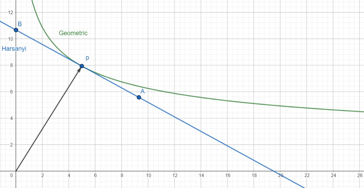
It's easy to find the points $s\in R^n$ which have the same $G$ score as $p$: they're the points which satisfy $G(s,\psi )=G(p,\psi )$. They all lie on a skewed hyperbola that touches $P$ at $p$.

One way to think about $G$ is as a hypersurface in $n+1$-dimensional space sitting "above" the n-dimensional space of utilities we've been working with. When there are 2 agents, we can plot $G$ using the third vertical axis.

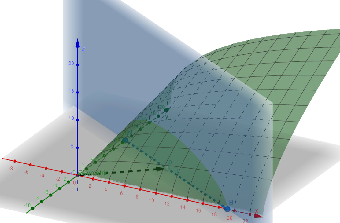
Check out the intersection of $G$ and the vertical plane above the Harsanyi line $H$: this tells us about the values of $G$ along this line, and as we shift $p$ we can recalculate $\psi$ so that among $H$, $G$ peaks at $p$.

Our choice of $p$ determines where we land on that surface "above" p. If we take a slice through $G$ by only looking at the points of $G$ at the same "altitude" as $p$, we get exactly that hyperbola back! 

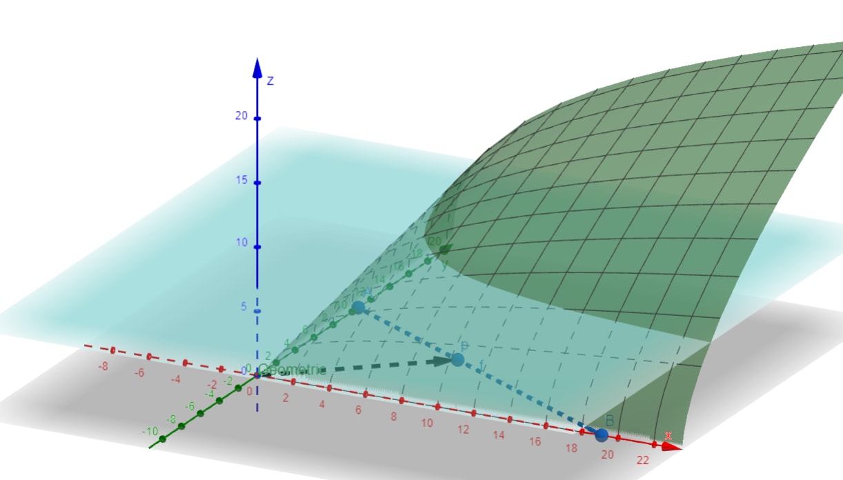
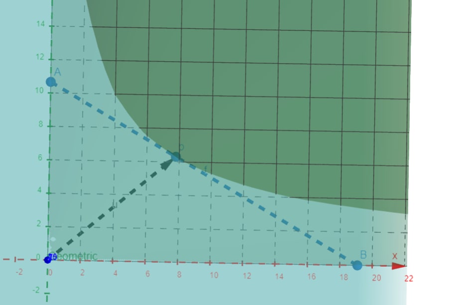
Doing this for many altitudes gives us a contour map, which you're probably familiar with in the context of displaying the altitude of real 3D landscapes on flat 2D maps.

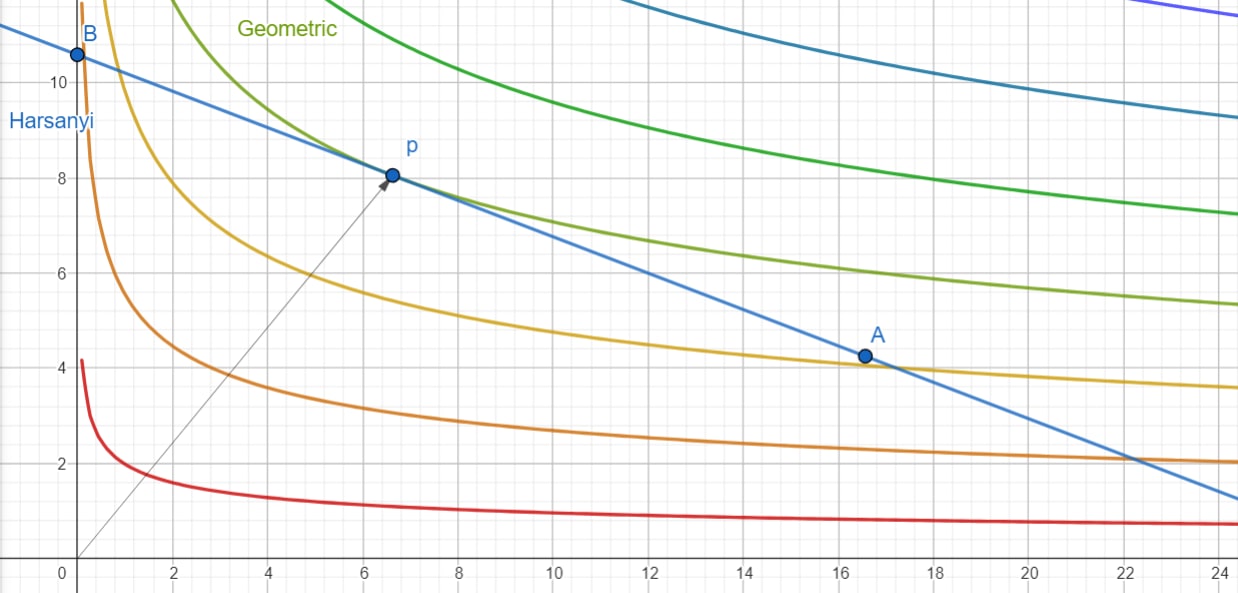
You can see how these contours change as we change $p$ and $H$ using the interactive version here.

There's a theorem which tells us that the gradient of $G$ must either be 0 or perpendicular to these contour hypersurfaces. So by calculating the gradient, we can calculate the tangent hyperplane of our skewed hyperbolas! And then we'll see if anything interesting happens at $p$.

This is a subproblem of the gradient calculation we did earlier [LW · GW], where we were specifically interested in how $G$ changes along the Harsanyi hyperplane $H$. The slope of $H$, encoded in $\varphi (p,F)$, showed up in how we defined $\psi (p,F)$. So let's see how $\varphi$ and $p$ have shaped the geometry of $G(\_,\psi )$.

The gradient ${\nabla }_{u}G(u,\psi )$ is just a vector of partial derivatives ${\nabla }_u{G}_i(u,\psi )=\frac{\partial G}{\partial u_i}$, where we're using ${\nabla }_u$ to remind ourselves that this is just the gradient with respect to $u$, holding $\psi$ constant. We're holding the weights constant, and $u$ isn't a function this time where we'd need to use the chain rule, so all we need to do is apply the power rule:

$\frac{\partial G}{\partial u_i}(u,\psi )=\frac{\partial }{\partial u_i}G(u,\psi )$

$\frac{\partial G}{\partial u_i}(u,\psi )=\frac{\partial }{\partial u_i}\left({\prod }_{j=1}^n{u}_j^{{\psi }_j}\right)$

$\frac{\partial G}{\partial u_i}(u,\psi )={\psi }_i{u}_i^{{\psi }_i-1}{\prod }_{j=1,j\ne i}^n{u}_j^{{\psi }_j}$

$\frac{\partial G}{\partial u_i}(u,\psi )=\frac{{\psi }_i}{u_i}{u}_i^{{\psi }_i}{\prod }_{j=1,j\ne i}^n{u}_j^{{\psi }_j}$

$\frac{\partial G}{\partial u_i}(u,\psi )=\frac{{\psi }_i}{u_i}{\prod }_{j=1}^n{u}_j^{{\psi }_j}$

$\frac{\partial G}{\partial u_i}(u,\psi )=\frac{{\psi }_i}{u_i}G(u,\psi )$

If we use $\oslash$ to denote element-wise division, this gives us a simple formula for ${\nabla }_{u}G$:

${\nabla }_{u}G=(\psi \oslash u)G$

or a component

${\nabla }_u{G}_i=\frac{{\psi }_i}{u_i}G$

And that's it! ${\nabla }_{u}G$ is defined when $u_i>0$ for all agents. Where ${\nabla }_{u}G$ is defined, we can keep taking derivatives; $G(u,\psi )$ is smooth everywhere $u_i>0$ for all agents.

Here's what it looks like!

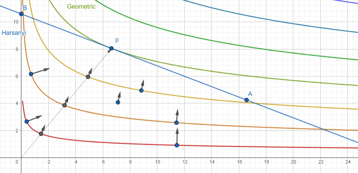
Playing around with an interactive version, you can see that as you approach giving an agent 0 utility, the gradient arrow gets longer and longer. As long as ${\psi }_i>0$, ${\nabla }_u{G}_i$ diverges off to infinity as $u_i$ approaches 0. When ${\psi }_i=0$, changing $u_i$ doesn't change $G$ and ${\nabla }_u{G}_i=0$.

Normatively, $G$ being 0 whenever any individual utility is 0 is a nice property to have. As long as we give an agent some weight, there is a pressure towards giving them more utility. If you've gotten this far you've probably taken a calculus class, and you probably studied how to enclose the largest area using a fixed perimeter of fencing. This is exactly the same pressure pushing us towards squares and away from skinny rectangles. The Pareto optima are points where the pressures favoring each agent balance, for some weights $\psi$, and we can design $\psi$ to cause all those pressures to balance at any point we choose along the Pareto frontier.

The visual analogy between "maximizing a product" and "sliding a hyperbola until it reaches the Pareto frontier" was really helpful in thinking about this problem. I first learned about that lens from Abram Demski's [LW · GW] great Comparing Utilities [LW · GW] post, which included illustrations by Daniel Demski that really helped me visualize what was going on as we maximize $G$.

Another thing we can notice is that $\nabla G_i\ge 0$. This is exactly what we'd expect from a Pareto monotone aggregation function. Geometrically, this means those contour lines always get further and further away from $F$, and they don't curve back in to make some other point in $F$ score higher on $G(\_,\psi )$ than $p$.

Gradient Ascent

The simplest proof I've found that goes from

• $p$ maximizes $G(\_,\psi )$ among $H$

to

• $p$ maximizes $G(\_,\psi )$ among $F$ 

relies on the fact that, if you start inside $F$ and follow the gradient ${\nabla }_{u}G$ to make $G$ larger and larger, you'll eventually run into the Harsanyi hyperplane $H$. In order for this to be true, ${\nabla }_{u}G$ needs to point at least a little bit in the direction perpendicular to $H$.

The Normal Vector to The Harsanyi Hyperplane

What is that direction? One way to think about $H$ is as a contour hyperplane of $H$, the Harsanyi aggregation function. $H$ is all of the joint utilities $u\in R^n$ where $H(u,\varphi )=H(p,\varphi )$. We know that the gradient ${\nabla }_{u}H$ will be perpendicular to this contour hyperplane, so let's compute that in order to find the normal vector to $H$:

$\frac{\partial H}{\partial u_i}=\frac{\partial }{\partial u_i}\left({\sum }_{j=1}^n{u}_j{\varphi }_j\right)$

$\frac{\partial H}{\partial u_i}={\varphi }_i$

${\nabla }_u{H}_i={\varphi }_i$

It would make my tensor calculus teacher too sad for me to write that ${\nabla }_{u}H=\varphi$, but the components of the vector ${\nabla }_{u}H$ are always the same as the components of the covector $\varphi$. We can then normalize ${\nabla }_{u}H$ to get the normal vector to $H$ which I'll denote $h$:

$h_i=\frac{{\varphi }_i}{|\varphi |}$

$h=\frac{\varphi }{|\varphi |}$

The distinction isn't important for most of this sequence, but I do want to use different alphabets to keep track of which objects are vectors and which are maps from vectors to scalars because they're different geometric objects with different properties. If we decide to start measuring one agent's utility in terms of milli-utilons, effectively multiplying all of their utility measurements by 1,000, the component of that agent's Harsanyi weight ${\varphi }_i$ scales inversely in a way that perfectly cancels out this change. The slope of a line doesn't change when we change the units we use to measure it.

Gradient Ascenders Reach H

One way to think about the dot product is as a tool for measuring the lengths of vectors and the angles between them. If the dot product ${\nabla }_{u}G\cdot h$ is ever 0, it means that a gradient ascender will not be moving towards or away from $H$ at that point. There are $n-1$ such orthogonal directions available, so for our proof to work we need to check that our choice of $\psi$ always leads to movement towards or away from $H$. Let's see what it takes to satisfy ${\nabla }_{u}G\cdot h=0$

${\nabla }_{u}G\cdot h=0$

${\sum }_{i=1}^n\left({\nabla }_u{G}_i\right)h_i=0$

${\sum }_{i=1}^n\left(\frac{{\psi }_i}{u_i}G\right)\frac{{\varphi }_i}{|\varphi |}=0$

All of these terms are non-negative, so in order for ${\nabla }_{u}G\cdot h$ to be 0, each element of this sum needs to be simultaneously 0. Can this happen for our choice of $\psi$?

${\psi }_i=\frac{p_i{\varphi }_i}{p\cdot \varphi }$

$\left(\frac{p_i{\varphi }_i}{u_i(p\cdot \varphi )}G\right)\frac{{\varphi }_i}{|\varphi |}=0$

We know that ${\varphi }_i>0$ for at least one agent $i$, and that if $p_i=0$ for all agents, that the entire Pareto frontier must consist only of that point at the origin. (In which case all choices of $\varphi$ and $\psi$ make that point optimal, and any gradient ascender will trivially find the optimum.) Otherwise, wherever ${\nabla }_{u}G$ is defined it points at least a little in the same direction as $h$. (And where it's not defined, it's because some component has diverged off to positive infinity because $u_i=0$ for some agent.)

In other words, using our choice of $\psi$, all gradient ascenders will either stay at their initial local minimum (because they were placed on a part of the boundary of $F$ where $G=0$ and ${\nabla }_{u}G$ is undefined), or they will eventually reach the Harsanyi hyperplane.

This is also a great time to point out that

 ${\nabla }_u{G}_i(p,\psi )=\frac{{\psi }_i}{p_i}G(p,\psi )=\frac{p_i{\varphi }_i}{p_i(p\cdot \varphi )}G(p,\psi )$

When $p_i>0$ for all agents, ${\nabla }_{u}G$ points in the same direction as $\varphi$ at $p$. This is a direct consequence of choosing $\psi$ such that ${\nabla }_{u}G$ is perpendicular to $H$. So $H$ is the tangent hyperplane to the Pareto frontier at $p$. But $G(\_,\psi )$ has been designed so that $H$ is also the tangent hyperplane to the contour curve of $G$ at $p$.

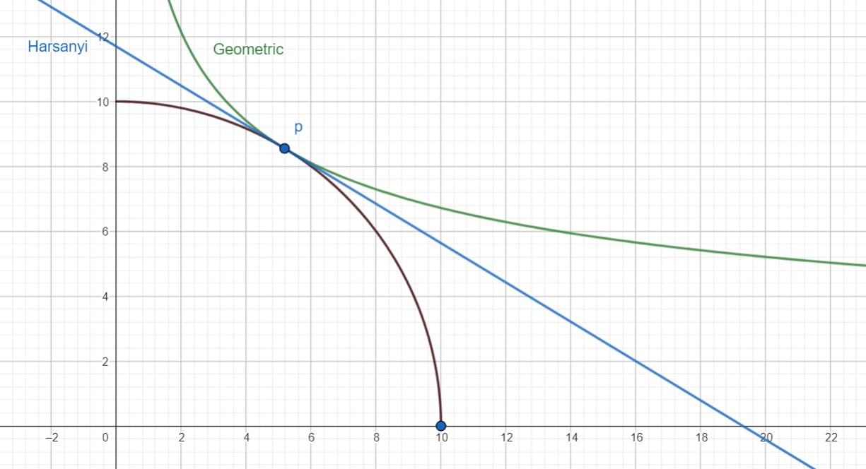
You can play with an interactive version here!

0 comments

Comments sorted by top scores.