A Solomonoff Inductor Walks Into a Bar: Schelling Points for Communication

post by johnswentworth, David Lorell · 2024-07-26T00:33:42.000Z · LW · GW · 0 comments

Contents

  Main Tool: Natural Latents for Minimum Description Length
    Fundamental Theorem
      The Intuition
      Background: Working with Kolmogorov Complexity
      More Precise Statement of the Fundamental Theorem
    Implications: Minimality, Maximality, Isomorphism
      Minimality
      Maximality
      Isomorphism
    Main Takeaway
  Back to Solomonoff’s Bar
      Even Simpler Subproblem: Just One Drink Type
    Multiple Drink Types: Categorizing by Shared Natural Latent
      Formal Specification
  Conclusion & Takeaways
  Appendix: Proof of the Fundamental Theorem
    Interpretation & Manipulation of Diagrams
      The Dangly Bit Lemma
      Re-Rooting of Markov Chains
      Marginalization in Markov Chains
    Proof of the Fundamental Theorem
      Mediation -> Graph
      Redundancy -> Graph
      The Graphical Part
None
No comments

A Solomonoff inductor walks into a bar in a foreign land. (Stop me if you’ve heard this one before.) The bartender, who is also a Solomonoff inductor, asks “What’ll it be?”. The customer looks around at what the other patrons are having, points to an unfamiliar drink, and says “One of those, please.”. The bartender points to a drawing of the same drink on a menu, and says “One of those?”. The customer replies “Yes, one of those.”. The bartender then delivers a drink, and it matches what the first inductor expected.

What’s up with that?

The puzzle, here, is that the two Solomonoff inductors seemingly agree on a categorization - i.e. which things count as the Unnamed Kind Of Drink, and which things don’t, with at least enough agreement that the customer’s drink-type matches the customer’s expectations. And the two inductors reach that agreement without learning the category from huge amounts of labeled data - one inductor points at an instance, another inductor points at another instance, and then the first inductor gets the kind of drink it expected. Why (and when) are the two inductors able to coordinate on roughly the same categorization?

Most existing work on Solomonoff inductors, Kolmogorov complexity, or minimum description length can’t say much about this sort of thing. The problem is that the customer/bartender story is all about the internal structure of the minimum description - the (possibly implicit) “categories” which the two inductors use inside of their minimal descriptions in order to compress their raw data. The theory of minimum description length typically treats programs as black boxes, and doesn’t attempt to talk about their internal structure.

In this post, we’ll show one potential way to solve the puzzle - one potential way for two minimum-description-length-based minds to coordinate on a categorization.

Main Tool: Natural Latents for Minimum Description Length

Fundamental Theorem

Here’s the main foundational theorem we’ll use. (Just the statement for now, more later.)

We have a set of n data points (binary strings) $\left\{x_i\right\}$, and a Turing machine TM. Suppose we find some programs/strings $\Lambda ,\left\{{\varphi }_i\right\},{\Lambda }^{\prime },\left\{{\varphi }_i^{\prime }\right\}$ such that:

• Mediation: $(\Lambda ,{\varphi }_1,\dots ,{\varphi }_n)$ is an approximately-shortest string such that (TM($\Lambda ,{\varphi }_i$) = $x_i$ for all $i$)
• Redundancy: For all $i$, $({\Lambda }^{\prime },{\varphi }_i^{\prime })$ is an approximately-shortest string such that TM(${\Lambda }^{\prime },{\varphi }_i^{\prime }$) = $x_i$.^[1]

Then: the K-complexity of ${\Lambda }^{\prime }$ given $\Lambda ,K\left({\Lambda }^{\prime }|\Lambda \right)$, is approximately zero - in other words, ${\Lambda }^{\prime }$ is approximately determined by $\Lambda$, in a K-complexity sense.

(As a preview: later we’ll assume that both $\Lambda$ and ${\Lambda }^{\prime }$ satisfy both conditions, so both $K\left({\Lambda }^{\prime }|\Lambda \right)$ and $K\left(\Lambda |{\Lambda }^{\prime }\right)$ are approximately zero. In that case, $\Lambda$ and ${\Lambda }^{\prime }$ are “approximately isomorphic” in the sense that either can be computed from the other by a short program. We’ll eventually tackle the customer/bartender puzzle from the start of this post by suggesting that $\Lambda$ and ${\Lambda }^{\prime }$ each encode a summary of things in one category according to one inductor, so the theorem then says that their category summaries are “approximately isomorphic”.)

The Intuition

What does this theorem mean intuitively?

Let’s start with the first condition: $(\Lambda ,{\varphi }_1,\dots ,{\varphi }_n)$ is an approximately-shortest string such that (TM($\Lambda ,{\varphi }_i$) = $x_i$ for all $i$). Notice that there’s a somewhat-trivial way to satisfy that condition: take $\Lambda$ to be a minimal description of the whole dataset $\left\{x_i\right\}$, take ${\varphi }_i=i$, and then add a little bit of code to $\Lambda$ to pick out the datapoint at index ${\varphi }_i$^[2]. So TM($\Lambda ,{\varphi }_i$) computes all of $\left\{x_i\right\}$ from $\Lambda$, then picks out index $i$. Now, that might not be the only approximately-minimal description (though it does imply that whatever approximately-minimal $\Lambda ,\varphi$ we do use is approximately a minimal description for all of x). Conceptually, insofar as there’s information in $x_i$ which is irrelevant to all the other $x_j$’s, we could “move” that information from $\Lambda$ into ${\varphi }_i$. But any information which is relevant to more than one $x_i$ has to be in $\Lambda$.

Now let’s consider the second condition: for all $i$, $({\Lambda }^{\prime },{\varphi }_i^{\prime })$ is an approximately-shortest string such that TM(${\Lambda }^{\prime },{\varphi }_i^{\prime }$) = $x_i$. Again, there’s a somewhat-trivial way to satisfy the condition: take ${\Lambda }^{\prime }$ to be empty, and ${\varphi }_i^{\prime }$ to be a minimal description of $x_i$. Again, that might not be the only approximately-minimal description. Conceptually, insofar as there’s information which is redundantly represented across all the $x_i$’s, that information can be “moved” into ${\Lambda }^{\prime }$. But ${\Lambda }^{\prime }$ can only contain information which is redundantly represented across all $x_i$’s.

Put those two together, and we get a simple intuitive statement of the theorem: if $\Lambda$ contains all information which is relevant to more than one datapoint, and ${\Lambda }^{\prime }$ contains only information which is redundantly represented across all datapoints, then $\Lambda$ contains all the information in ${\Lambda }^{\prime }$.

Intuitively: imagine that $\Lambda$ is a pipe between $x_i$ and $x_j$, and the only way for information to move between $x_i$ and $x_j$ is through that pipe. Then if some information ${\Lambda }^{\prime }$ is present in both $x_i$ and $x_j$, it must have gone through the pipe. It’s the same idea as deterministic natural latents [LW · GW], but now in a minimum description length setting.

So that’s the idea. Now we’re ready for the actual math.

Background: Working with Kolmogorov Complexity

We kicked around the word “approximation” a lot, in stating the theorem. Approximation in what sense?

When working with Kolmogorov complexity, a prototypical theorem looks like:

• Take in the value of some K-complexity, $K\left(X|Y\right)$. That means assuming there exists a program of length $K\left(X|Y\right)$ which outputs $X$ on input $Y$. Call that program $F$ (for “function”).
• Construct some other program $F^{\prime }$ which either uses $F$ as a subroutine, or relies somehow on the existence of $F$. The length of the new program is either the length of $F$ (i.e. $K\left(X|Y\right)$) plus a little bit of new code, or just a little bit of new code. The theorem says the new code is small in a big-$O$ sense compared to the length of $F$ - i.e. $O\left(1\right)$ or $O\left(\text{log}K\right(X|Y\left)\right)$ is typical.

As an example: if $Y$ is a shortest program to compute $X$, then

$K\left(Y|X\right)\le O($log $K\left(X\right))$ ^[3]

Here’s a rough sketch of the program of size $O($log $K\left(X\right))$ which outputs $Y$ on input $X$. The program will have $K\left(X\right)$ hardcoded (which takes $O($log $K\left(X\right))$ bits). It will also have hardcoded a number $k$, such that among inputless programs of size $K\left(X\right)$ which output $X$, $Y$ is the $k^{th}$ to halt. It turns out that there can’t be very many minimal programs (though we won’t prove that part here), so log $k\le O($log $K\left(X\right))$. The program itself runs all programs of length $K\left(X\right)$ until the $k^{th}$ halts and returns $X$, then returns the $k^{th}$ program to halt and return $X$; that code requires only a constant number of bits to specify. So, the total size of the program is $O($log $K\left(X\right))$ bits.

That’s what the programs involved in prototypical K-complexity theorems tend to look like. The key idea to remember is that, wherever you see O(blah) terms, that usually means there’s some simple wrapper code of the relevant size.

More Precise Statement of the Fundamental Theorem

We have a set of $n$ data points (binary strings) $\left\{x_i\right\}$, and a Turing machine TM. Suppose we find some programs/strings $\Lambda ,\left\{{\varphi }_i\right\},{\Lambda }^{\prime },\left\{{\varphi }_i^{\prime }\right\}$ such that:

• Mediation: len($\Lambda ,{\varphi }_1,\dots ,{\varphi }_n$) $\le ϵ+$ min${}_{\Lambda ,{\varphi }_1,\dots ,{\varphi }_n}$ len($\Lambda ,{\varphi }_1,\dots ,{\varphi }_n$) subject to (TM($\Lambda ,{\varphi }_i$) = $x_i$ for all $i$)
• Redundancy: For all $i$, len(${\Lambda }^{\prime },{\varphi }_i^{\prime }$) $\le {ϵ}^{\prime }+$min${}_{{\Lambda }^{\prime },{\varphi }_i^{\prime }}$ len(${\Lambda }^{\prime },{\varphi }_i^{\prime }$) subject to TM(${\Lambda }^{\prime },{\varphi }_i^{\prime }$) = $x_i$.

Then: $O($$ϵ+{ϵ}^{\prime }+$log $K\left(x\right)$) $\ge K\left({\Lambda }^{\prime }|\Lambda \right)$.

The proof has been relegated to the appendix.

Implications: Minimality, Maximality, Isomorphism

When a string $\Lambda$ satisfies both the mediation and redundancy conditions over some strings $x_1,\dots ,x_n$, we call $\Lambda$ a natural latent over $x_1,\dots ,x_n$ (overloading our terminology for "natural latents" in the probabilistic setting). Equipped with the fundamental theorem, we can now carry over all the standard properties of deterministic natural latents [LW · GW] in the probabilistic setting to natural latents in the minimum description length setting.

Minimality

Suppose the string $\Lambda$ satisfies both the mediation and redundancy conditions over some strings $x_1\dots x_n$:

• Mediation: there exists ${\varphi }_1,\dots ,{\varphi }_n$ such that $(\Lambda ,\varphi )$ has minimal length to within $ϵ$ bits subject to ($\forall i$: TM($\Lambda ,{\varphi }_i$) = $x_i$).
• Redundancy: For all $i$, there exists ${\varphi }_i^{\prime }$ such that ($\Lambda ,{\varphi }_i^{\prime }$) has minimal length to within ${ϵ}^{\prime }$ bits subject to TM($\Lambda ,{\varphi }_i^{\prime }$) = $x_i$.

Then  $\Lambda$ satisfies the mediation condition, and for any other string ${\Lambda }^{\prime }$ which satisfies the mediation condition to within $ϵ$ bits, the Fundamental Theorem tells us

$O(ϵ+{ϵ}^{\prime }+$ log $K(x_1,x_2))\ge K(\Lambda |{\Lambda }^{\prime })$

i.e. there exists a short program to compute $\Lambda$ from ${\Lambda }^{\prime }$. So $\Lambda$ is a “minimal” string which satisfies the mediation condition; it can be computed from any other via a short program.

Maximality

Suppose, again, that the string $\Lambda$ satisfies both the mediation and redundancy conditions over some strings $x_1\dots x_n$:

• Mediation: there exists ${\varphi }_1,\dots ,{\varphi }_n$ such that $(\Lambda ,\varphi )$ has minimal length to within $ϵ$ bits subject to ($\forall i$: TM($\Lambda ,{\varphi }_i$) = $x_i$).
• Redundancy: For all $i$, there exists ${\varphi }_i^{\prime }$ such that $(\Lambda ,{\varphi }_i^{\prime })$ has minimal length to within ${ϵ}^{\prime }$ bits subject to TM($\Lambda ,{\varphi }_i^{\prime }$) = $x_i$.

Then $\Lambda$ satisfies the redundancy condition, and for any other string ${\Lambda }^{\prime }$ which satisfies the redundancy condition to within ${ϵ}^{\prime }$ bits, the Fundamental Theorem tells us

$O(ϵ+{ϵ}^{\prime }+$ log $K(x_1,x_2))\ge K({\Lambda }^{\prime }|\Lambda )$

i.e. there exists a short program to compute ${\Lambda }^{\prime }$ from $\Lambda$. So $\Lambda$ is a “maximal” string which satisfies the redundancy condition; any other can be computed from $\Lambda$ via a short program.

Isomorphism

Finally, suppose that both the string $\Lambda$ and the string ${\Lambda }^{\prime }$ satisfy both mediation and redundancy to within \epsilon and \epsilon’ bits, respectively. Then

$O(ϵ+{ϵ}^{\prime }+$ log $K(x_1,x_2))\ge K(\Lambda |{\Lambda }^{\prime })$

and 

$O(ϵ+{ϵ}^{\prime }+$ log $K(x_1,x_2))\ge K({\Lambda }^{\prime }|\Lambda )$

So either of the strings $\Lambda ,{\Lambda }^{\prime }$ can be computed from the other via a short program. In that sense, the two are “isomorphic”.

Main Takeaway

The main upshot which we’ll use in the next section is the isomorphism property, so we’ll restate it here in full.

Suppose the string $\Lambda$ satisfies both the mediation and redundancy conditions over some strings $x_1\dots x_n$:

• Mediation: there exists ${\varphi }_1,\dots ,{\varphi }_n$ such that $(\Lambda ,\varphi )$ has minimal length to within $ϵ$ bits subject to ($\forall i$: TM($\Lambda ,{\varphi }_i$) = $x_i$).
• Redundancy: For all $i$, there exists ${\varphi }_i^{\prime }$ such that $(\Lambda ,{\varphi }_i^{\prime })$ has minimal length to within ${ϵ}^{\prime }$ bits subject to TM($\Lambda ,{\varphi }_i^{\prime }$) = $x_i$.

Assume that ${\Lambda }^{\prime }$ also satisfies both conditions:

• Mediation: there exists ${\varphi }_1,\dots ,{\varphi }_n$ such that $({\Lambda }^{\prime },\varphi )$ has minimal length to within $ϵ$ bits subject to ($\forall i$: TM(${\Lambda }^{\prime },{\varphi }_i$) = $x_i$).
• Redundancy: For all $i$, there exists ${\varphi }_i^{\prime }$ such that $({\Lambda }^{\prime },{\varphi }_i^{\prime })$ has minimal length to within ${ϵ}^{\prime }$ bits subject to TM(${\Lambda }^{\prime },{\varphi }_i^{\prime }$) = $x_i$.

Intuitively, these say that both $\Lambda$ and ${\Lambda }^{\prime }$ capture approximately all the information which is relevant to more than one $x_i$, and approximately only the information which is redundantly represented across all $x_i$.

Then:

$O(ϵ+{ϵ}^{\prime }+$ log $K(x_1,x_2))\ge K(\Lambda |{\Lambda }^{\prime })$

$O(ϵ+{ϵ}^{\prime }+$ log $K(x_1,x_2))\ge K({\Lambda }^{\prime }|\Lambda )$

In other words: a short program exists to compute $\Lambda$ from ${\Lambda }^{\prime }$, and a short program exists to compute ${\Lambda }^{\prime }$ from $\Lambda$.

Back to Solomonoff’s Bar

Let’s talk about the problem faced by our two Solomonoff inductors - the customer and the bartender.

As a (very) simplified model, let’s say that they both start out with matching background models of what generally happens when one places an order in a bar - i.e. certain words are spoken, a liquid shows up in a container, all that jazz. We’ll assume that the two already break up the world into a bunch of individual instances of “drinks” (a pint on the bar over here, a glass on the table over there, …) all of which are observed by both inductors; that will be our most egregious simplification of the problem. We’ll call those individual drink-instances in the world $x_1,\dots ,x_n$. The (very simplified) problem the two then face is how to categorize various physical instances of liquids-in-containers, such that when the customer asks for a drink in a certain category (i.e. “one of those” + pointing), they end up with the kind of drink they expected.

By contrast, what would be a bad outcome for the two? Well, maybe the bartender just categorizes drinks by booze content, and the customer just categorizes drinks by color, so the customer thinks they’re asking for a blue drink but the bartender thinks they’re asking for a drink with 10% alcohol content, and the customer unexpectedly-to-them ends up with a pink drink. That’s the sort of thing we want to avoid.

So the customer and the bartender face a coordination problem - both want the customer to not be surprised at their drink. And it’s a coordination problem in the Schelling sense [LW · GW], insofar as the two will not be able to exchange anywhere near enough data to brute-force learn each others’ categorizations.

How can the two use the theorems here to coordinate on a choice of categorization, without exponentially huge amounts of communication? We’ll tackle the problem in two steps:

• First, an even simpler problem in which there’s just one drink type, in order to illustrate what parts of the problem are handled by the isomorphism argument.
• Second, the simplified customer/bartender problem itself, with multiple drink types.

Even Simpler Subproblem: Just One Drink Type

Suppose there’s just one drink type - maybe this is soviet Russia, and a shot of vodka is the only option. We still have a version of the customer/bartender problem: they should both roughly agree on what a shot of vodka is. If the bartender prepares a thing which they think of as a shot of vodka, the customer should not receive a thing which they think of as, say, a giraffe.

Well, both inductors see $x_1,\dots ,x_n$, which are all shot-of-vodka-instances. Suppose they both look for a natural latent over those instances, and both find one: $\Lambda$ for the customer, ${\Lambda }^{\prime }$ for the bartender. Then we know that the two have found approximately-isomorphic strings.

Now, the bartender creates a new thing $x_{n+1}$, which is approximately-optimally compressed as passing a new incompressible string (i.e. noise) to the generator ${\Lambda }^{\prime }$, just like the bartender models all the other $x_i$’s as having been generated. ${\Lambda }^{\prime }$ is therefore natural over $x_1,\dots ,x_{n+1}$. And since ${\Lambda }^{\prime }$ is approximately isomorphic to $\Lambda$, $\Lambda$ is natural over $x_1,\dots ,x_{n+1}$. So, when the customer receives their drink, they see that it’s approximately-optimally compressed by $\Lambda$ plus some incompressible noise, and it’s also approximately-optimally compressed jointly with $x_1,\dots ,x_n$ by $\Lambda$ plus some incompressible noise. It is, in other words, basically what the customer expected.

So that’s the basic story. Now let’s kick it up a notch, and handle multiple drink-types.

Multiple Drink Types: Categorizing by Shared Natural Latent

Our two inductors both start out with the “data points” $x_1,\dots ,x_n$, each of which is one physical instance of a drink. Then one obvious move is to look for a natural latent over these strings, or over various subsets of the strings.

In general, there’s no guarantee that any natural latent exists at all (to within reasonable approximation). And even if natural latents do exist over some subsets of the data points, they might have some complicated structure - e.g. maybe there’s a natural latent between $x_1$ and $x_2$ and another between $x_2$ and $x_3$ but those two have very different stuff in them, or maybe there’s hierarchical structure like e.g. a natural latent over the first half of the data and another over the second half and then a natural latent over those two natural latents, or ???. Most of those possibilities don’t look much like “categories of drinks”, at least not in a simple sense. But perhaps our intuitive notion of simple “categories” maps to a specific kind of natural latent structure?

Here’s a simple structure which seems like a decent fit.

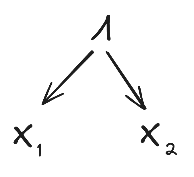
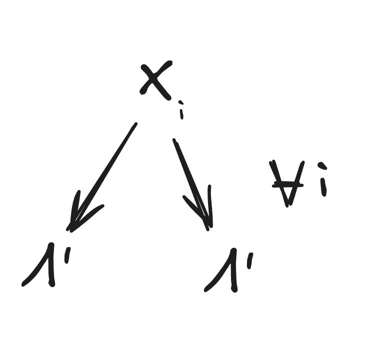
Imagine that we have 8 drink-instances $x_1,\dots ,x_8$. We find a natural latent ${\Lambda }_a$ between $x_1$ and $x_2$. On further investigation, we find that the same string ${\Lambda }_a$ is natural over all of $x_1,x_2,x_5$, and $x_7$.^[4] Then we find another string ${\Lambda }_b$which is natural over $x_3$ and $x_4$, and a third string ${\Lambda }_c$ which is natural over $x_6$ and $x_8$. Finally, we find that the strings $\{x_1,x_2,x_5,x_7\}$ are independent^[5] of the strings $\{x_3,x_4\}$ and all those are independent of the strings $\{x_6,x_8\}$.

We can summarize all that with the diagrams:

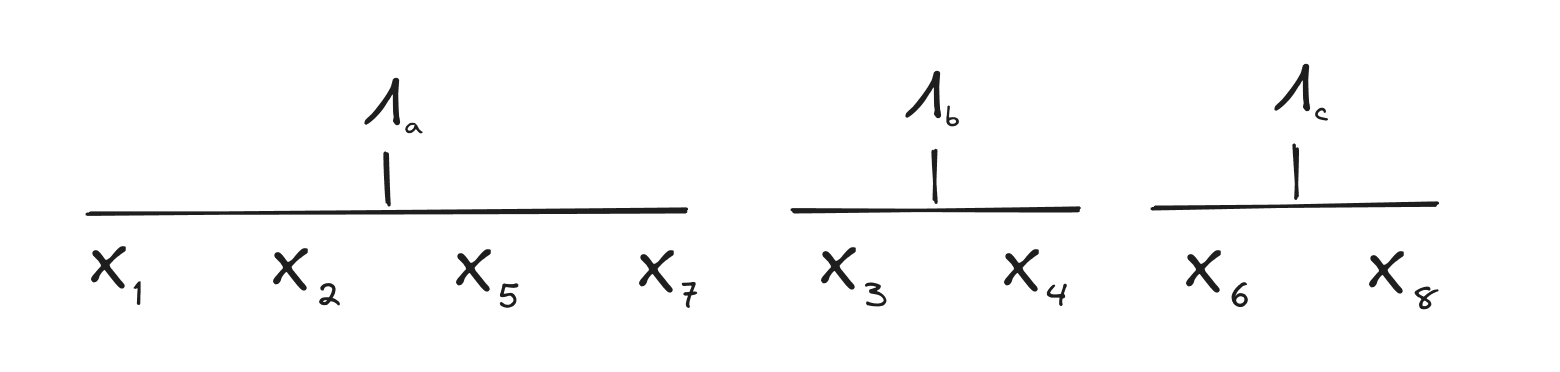
where we use the “$\perp$” symbol to denote naturality, and unconnected diagrams next to each other indicate independence.

In this case, it makes a lot of intuitive sense to view each of the three latents as a generator or specification for a certain category of drink. There is no compressible shared information across drinks in different categories, and ${\Lambda }_{\alpha }$ captures all-and-only the information shared across drinks with category $\alpha$, for each category $\alpha$.

If such $\Lambda$’s exist, how can the customer and bartender use them to solve their coordination problem?

Well, assume they’re both looking for $\Lambda$’s with this structure - i.e. they both want to partition the set of drinks such that there exists a nonempty natural latent over each subset, and independence^[6] across subsets. If that’s possible at all, then the partition is unique: pairwise independent strings must go in different subsets, and pairwise non-independent strings must go in the same subset. (If we consider a graph in which each node is one of the strings $x_i$ and two nodes are connected iff they are non-independent, then the connected components of that graph must be the subsets of the partition.)^[7]

With the partition nailed down, we next invoke uniqueness (up to isomorphism) of natural latents within each subset, i.e. the “isomorphism” result we proved earlier.^[8]

As long as the customer and bartender are both looking for this kind of structure in the strings $x_1,\dots ,x_n$, and the structure exists to be found in the strings, they will find the same partition (modulo approximation) and approximately isomorphic latents characterizing each class of drinks.

So the customer walks into the bar. They point at a drink - let’s say it’s $x_7$ - and say “One of those, please.”. The bartender has $x_7$ in subset $a$, with generator ${\Lambda }_a$. Just to double check, they point to a picture of a drink also generated by ${\Lambda }_a$, and the customer confirms that’s the type of drink they want. The bartender generates a drink accordingly. And since the customer and bartender have approximately isomorphic ${\Lambda }_a$, the customer gets what they expected, to within reasonable approximation.

Formal Specification

Both inductors look for

• some strings ${\Lambda }_1,\dots ,{\Lambda }_k$ (conceptually: ${\Lambda }_j$ encodes a generator for drink type $j$),
• integers $c_1,\dots ,c_n$ in $[1,\dots ,k]$ (conceptually: the category of each drink-instance),
• and bitstrings ${\varphi }_1,\dots ,{\varphi }_n,{\varphi }_1^{\prime },\dots ,{\varphi }_n^{\prime },{\varphi }_1^{\prime \prime },\dots ,{\varphi }_n^{\prime \prime }$ (conceptually: random noise encoding details of each drink-instance for each of the optimization problems)

such that

• Mediation: $({\Lambda }_{c^{\ast }},{\varphi }_{i:c_i=c^{\ast }})$ is minimal to within $ϵ$ subject to ($\forall i$ s.t. $c_i=c^{\ast }$: TM(${\Lambda }_{c_i},{\varphi }_i$) = $x_i$)
• Redundancy: For all $i$, $({\Lambda }_{c_i},{\varphi }_i^{\prime })$ is minimal to within ${ϵ}^{\prime }$ subject to TM(${\Lambda }_{c_i},{\varphi }_i^{\prime }$) = $x_i$
• Independence across categories: $(\Lambda ,{\varphi }^{\prime \prime })$ is minimal to within ${ϵ}^{\prime \prime }$ subject to ($\forall i$: TM(${\Lambda }_{c_i},{\varphi }_i^{\prime \prime }$) = $x_i$))

Note that all of these might be conditional on other background knowledge of the inductors - i.e. the Turing machine TM has access to a database full of all the other stuff the inductors know. However, they do need to condition only on things which they expect the other inductor to also know, since we’ve assumed the two inductors use the same Turing machine.^[9]

If you’ve been wondering why on Earth we would ever expect to find such simple structures in the complicated real world, conditioning on background knowledge is the main answer. Furthermore, our current best guess is that most of that background knowledge is also itself organized via natural latents, so that the customer and bartender can also coordinate on which knowledge to condition on.

Conclusion & Takeaways

First, let’s recap the core theorem of this post.

Suppose that some string $\Lambda$ satisfies both the following conditions over strings $x_1\dots x_n$ for a Turing machine TM:

• Mediation: there exists ${\varphi }_1,\dots ,{\varphi }_n$ such that $(\Lambda ,\varphi )$ has minimal length to within $ϵ$ bits subject to ($\forall i$: TM($\Lambda ,{\varphi }_i$) = $x_i$).
• Redundancy: For all $i$, there exists ${\varphi }_i^{\prime }$ such that $(\Lambda ,{\varphi }_i^{\prime })$ has minimal length to within ${ϵ}^{\prime }$ bits subject to TM($\Lambda ,{\varphi }_i^{\prime }$) = $x_i$.

Further, suppose that some string ${\Lambda }^{\prime }$ also satisfies those conditions over the same strings $x_1\dots x_n$ and Turing machine TM. Then:

$O(ϵ+{ϵ}^{\prime }+$ log $K(x_1,x_2))\ge K(\Lambda |{\Lambda }^{\prime })$

$O(ϵ+{ϵ}^{\prime }+$ log $K(x_1,x_2))\ge K({\Lambda }^{\prime }|\Lambda )$

In other words: a short program exists to compute $\Lambda$ from ${\Lambda }^{\prime }$, and a short program exists to compute ${\Lambda }^{\prime }$ from $\Lambda$.

Conceptually, we imagine two different agents each look for approximately-best compressions in the same form as the mediation and redundancy conditions. One agent finds $\Lambda$, one finds ${\Lambda }^{\prime }$. Then the two have found approximately isomorphic compressions.

Crucially, these are approximately isomorphic “parts of” compressions - i.e. they separate out “signal” $\Lambda$ from “noise” $\varphi$, and the two agents approximately agree on what the “signal” and “noise” each have to say about the data. So, they’ll approximately agree on what it would mean to sample new data points with the same “signal” but different random “noise” - e.g. the new drink-instance which the bartender prepares for the customer.

Conceptually, both the questions we tackle here and the methods used to answer it are similar to our semantics post [LW · GW], with two big differences. First, we’re now working with minimum description length rather than generic Bayesian probability, which means everything is uncomputable but conceptually simpler. Second, our method here for “multiple drink types” was actually totally different and non-analogous to the corresponding method [LW · GW] in the semantics post, even though the two methods used similar low-level tools (i.e. natural latents).^[10] One item for potential future work is to transport the method used in the semantics post over to the minimum description length context, and the method used in this post over to the generic Bayesian context. Another potential item is to unify the two; intuitively they seem closely related.

Our main hope is that other people will be able to pick up these methods and use them to characterize other kinds of concepts which different minds are able to converge upon and communicate about. We’ve only just scratched the surface here.

Appendix: Proof of the Fundamental Theorem

We’re going to use essentially the same diagrammatic proof as Deterministic Natural Latents [LW · GW] (don’t worry, we don’t assume you’ve read that). Of course, now we’re working with Kolmogorov complexity, so we have a new interpretation of each diagram, and we’ll need to prove all the diagrammatic rules we need to use.

Interpretation & Manipulation of Diagrams

Let’s start with an example diagram:

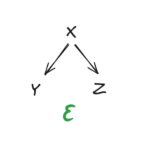
We say that this diagram “holds for” three strings $X$, $Y$, and $Z$ iff

$ϵ\ge K\left(X\right)+K\left(Y|X\right)+K\left(Z|X\right)-K(X,Y,Z)$

where $ϵ$ will often be a big-$O$ term.

More generally, a diagram is a directed acyclic graph in which each node $i$ is a string $X_i$, along with an error term $ϵ$. The diagram holds iff

$ϵ\ge {\sum }_{i}K\left(X_i|X_{pa\left(i\right)}\right)-K\left(X\right)$

where $pa\left(i\right)$ denotes the parents of node $i$ in the graph.

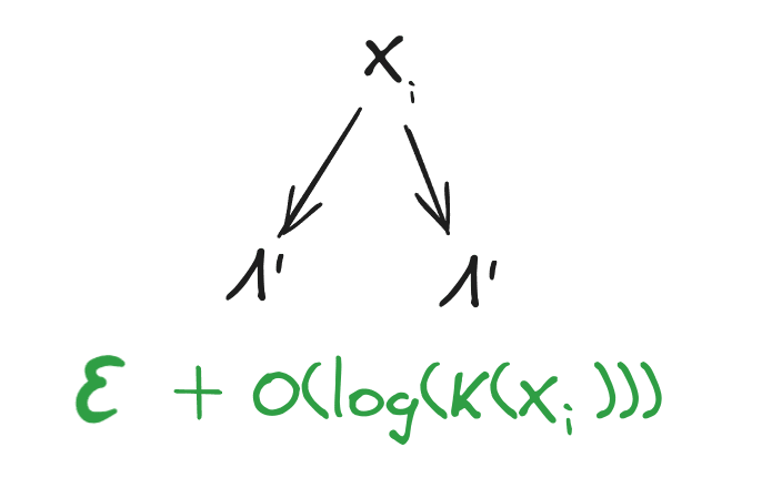
Note that the same string can appear more than once! For instance, the diagram

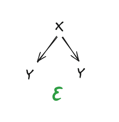
says that $ϵ\ge K\left(X\right)+K\left(Y|X\right)+K\left(Y|X\right)-K(X,Y,Y)$. Using the chain rule, that simplifies to

$O\left(\text{log}K\right(X,Y\left)\right)+ϵ\ge K\left(Y|X\right)$
i.e. $Y$ has only logarithmic complexity given $X$ (assuming the log term dominates $ϵ$). We’ll use diagrams like that one several times below, in order to indicate that one string has quite low complexity given another.

Now for some rules. We’ll need three:

• The Dangly Bit Lemma
• Re-Rooting of Markov Chains
• Marginalization in Markov Chains

The Dangly Bit Lemma

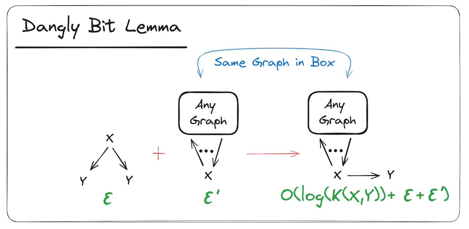
If $Y\leftarrow X\to Y$ holds to within $ϵ$ bits, and any other diagram $D$ involving $X$ holds to within ${ϵ}^{\prime }$ bits, then we can create a new diagram $D^{\prime }$ which is identical to $D$ but has another copy of $Y$ (the “dangly bit”) as a child of $X$. The new diagram $D^{\prime }$ will hold to within $ϵ+{ϵ}^{\prime }$ bits.

Proof (click to expand):

Assume the diagram $D$ is over $X$ and some other variables $Z$; it asserts that

${ϵ}^{\prime }\ge {\sum }_{i}K\left(\right(X,Z{)}_i|(X,Z{)}_{pa\left(i\right)})-K(X,Z)$

Since $Y\leftarrow X\to Y$ holds to within $ϵ$ bits,

$O($log $K(X,Y)+ϵ)\ge K(Y|X)$

(as shown in the previous section). Let’s add those two inequalities:

${ϵ}^{\prime }+O($log $K(X,Y)+ϵ)\ge K(Y|X)+{\sum }_{i}K((X,Z{)}_i|(X,Z{)}_{pa\left(i\right)})-K(X,Z)$

And since $K(X,Z)\le K(X,Y,Z)+O\left(1\right)$, we can replace the $K(X,Z)$ term to get

${ϵ}^{\prime }+O($log $K(X,Y)+ϵ)\ge K(Y|X)+{\sum }_{i}K((X,Z{)}_i|(X,Z{)}_{pa\left(i\right)})-K(X,Y,Z)$

which is the inequality asserted by the new diagram D’.

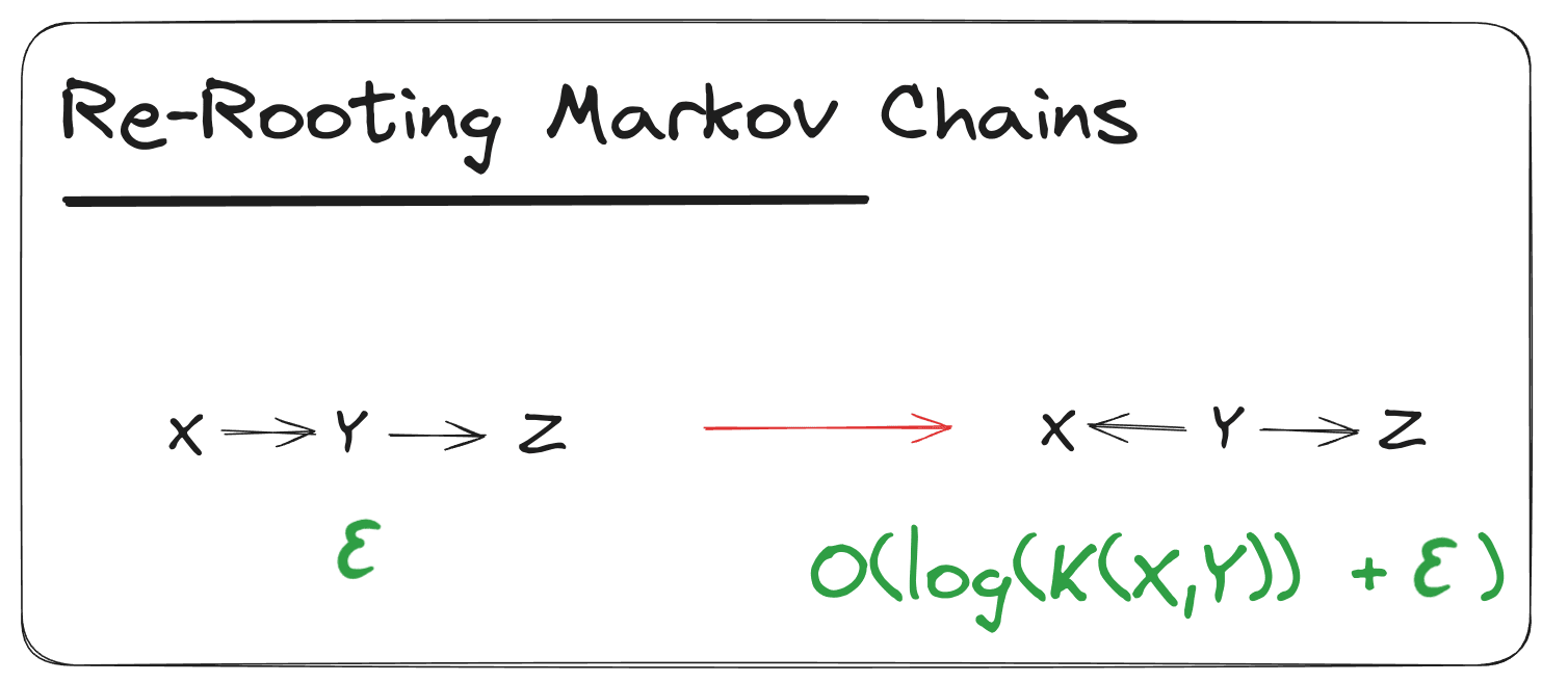
Re-Rooting of Markov Chains

Suppose we have a “Markov chain” diagram $X_1\leftarrow X_2\leftarrow \dots \leftarrow X_k\to \dots \to X_{n-1}\to X_n$ to within $ϵ$ bits. That diagram asserts

$ϵ\ge K\left(X_k\right)+{\sum }_{i<k}K\left(X_i|X_{i+1}\right)+{\sum }_{i>k}K\left(X_i|X_{i-1}\right)-K\left(X\right)$

Then we can move the root node right one step to form the diagram $X_1\leftarrow X_2\leftarrow \dots \leftarrow X_{k+1}\to \dots \to X_{n-1}\to X_n$ to within $ϵ+O($log $K(X_k,X_{k+1}))$ bits. Likewise for moving left one step.

Proof (click to expand):

We’ll do the proof for moving right one step, the proof for moving left one step works the same way.

$ϵ\ge K\left(X_k\right)+{\sum }_{i<k}K\left(X_i|X_{i+1}\right)+{\sum }_{i>k}K\left(X_i|X_{i-1}\right)-K\left(X\right)$

$=K\left(X_k\right)+K\left(X_{k+1}|X_k\right)+{\sum }_{i<k}K\left(X_i|X_{i+1}\right)+{\sum }_{i>k+1}K\left(X_i|X_{i-1}\right)-K\left(X\right)$

$\ge K(X_k,X_{k+1}|X_k)-O\left(1\right)+{\sum }_{i<k}K\left(X_i|X_{i+1}\right)+{\sum }_{i>k+1}K\left(X_i|X_{i-1}\right)-K\left(X\right)$

$\ge K\left(X_{k+1}\right)+K\left(X_k|X_{k+1}\right)-O\left(logK\right(X_k,X_{k+1}\left)\right)+{\sum }_{i<k}K\left(X_i|X_{i+1}\right)+{\sum }_{i>k+1}K\left(X_i|X_{i-1}\right)-K\left(X\right)$

$=K\left(X_{k+1}\right)+{\sum }_{i<k+1}K\left(X_i|X_{i+1}\right)+{\sum }_{i>k+1}K\left(X_i|X_{i-1}\right)-K\left(X\right)-O\left(logK\right(X_k,X_{k+1}\left)\right)$

By applying this rule repeatedly, we can arbitrarily re-root a Markov chain diagram.

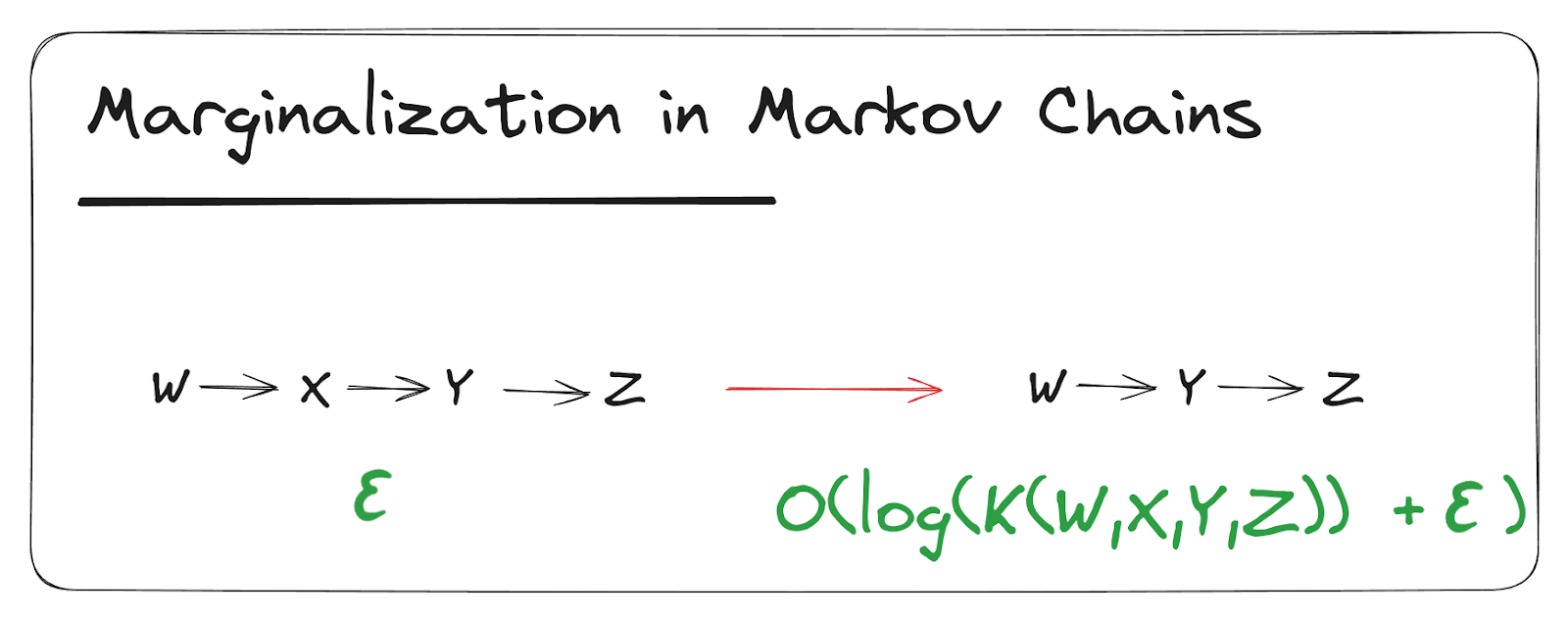
Marginalization in Markov Chains

Suppose the diagram $W\to X\to Y\to Z$ holds to within $ϵ$ bits. Then $W\to Y\to Z$ holds to within $ϵ+O($log $K(W,X,Y,Z))$ bits.

Proof (click to expand):

$ϵ\ge K\left(W\right)+K\left(X|W\right)+K\left(Y|X\right)+K\left(Z|Y\right)-K(W,X,Y,Z)$

$\ge K\left(W\right)+K\left(X|W\right)+K(Y|W,X)+K\left(Z|Y\right)-K(W,X,Y,Z)-O\left(1\right)$

$=K\left(Z|Y\right)-K(Z|W,X,Y)-O($log $K(W,X,Y,Z))$

$\ge K\left(Z|Y\right)-K(Z|W,Y)-O($log $K(W,X,Y,Z))$

$=K\left(W\right)+K\left(Y|W\right)+K\left(Z|Y\right)-K(W,Y,Z)-O($log $K(W,X,Y,Z))$

This proof also extends straightforwardly to longer Markov chains; that’s a good exercise if you’re looking for one.

When working with a longer chain $X_1\to \dots \to X_n$, note that reversing the direction of arrows in the Markov chain and further marginalization both also cost no more than $O($log $K\left(X\right))$, so we can marginalize out multiple variables and put the root anywhere for the same big-$O$ cost in the bounds.

Proof of the Fundamental Theorem

With all the foundations done, we’re now ready for the main proof. Here’s the full statement again:

We have a set of $n$ data points (binary strings) $\left\{x_i\right\}$, and a Turing machine TM. Suppose we find some programs/strings $\Lambda ,\left\{{\varphi }_i\right\},{\Lambda }^{\prime },\left\{{\varphi }_i^{\prime }\right\}$ such that:

• Mediation: len($\Lambda ,{\varphi }_1,\dots ,{\varphi }_n$) $\le ϵ+$min${}_{\Lambda ,{\varphi }_1,\dots ,{\varphi }_n}$ len($\Lambda ,{\varphi }_1,\dots ,{\varphi }_n$) subject to (TM($\Lambda ,{\varphi }_i$) = $x_i$ for all $i$)
• Redundancy: For all $i$, $({\Lambda }^{\prime },{\varphi }_i^{\prime })\le {ϵ}^{\prime }+$ min${}_{{\Lambda }^{\prime },{\varphi }_i^{\prime }}$ len(${\Lambda }^{\prime },{\varphi }_i^{\prime }$) subject to TM(${\Lambda }^{\prime },{\varphi }_i^{\prime }$) = $x_i$.

Then: $O(ϵ+{ϵ}^{\prime }+$log $K\left(x\right))\ge K({\Lambda }^{\prime }|\Lambda )$.

First, we’ll show that the mediation condition implies

and the redundancy condition implies

Following those two parts of the proof, the rest will proceed graphically.

Mediation -> Graph

Note that the mediation condition can always be satisfied to within $O(n$ log $n)$^[11] by taking $\Lambda$ to be a shortest program for $x$ plus $O\left(1\right)$ code to index into the result at position ${\varphi }_i$, and taking ${\varphi }_i=i$. So: 

1: If $(\Lambda ,\varphi )$ are to be minimal to within $ϵ$, they must satisfy len($\Lambda ,\varphi$) $\le K\left(x\right)+ϵ+O($log $K\left(x\right))$^[12]

Furthermore, for $(\Lambda ,\varphi )$ to be minimal to within $ϵ$ for anything: 

2: $(\Lambda ,\varphi )$  must themselves be incompressible to within that same $ϵ$: len($\Lambda ,\varphi$) $\le K(\Lambda ,\varphi )+ϵ+O($log $K(\Lambda ,\varphi ))$ = $K\left(x\right)+ϵ+O($log $K\left(x\right))$. As a corollary, $\Lambda$ and $\varphi$ must individually be incompressible to within that same bound or else together they couldn’t be minimal either.

Additionally note that ${\varphi }_i$ (plus some constant-size wrapper code) specifies $x_i$ given $\Lambda$, so:

3: $K\left(x_i|\Lambda \right)\le len\left({\varphi }_i\right)+O($log len(${\varphi }_i$)) = len(${\varphi }_i$) $+O($log K(X_i | \Lambda))

Now we put all that together.  (2) $\Lambda$ is incompressible to within $ϵ+O($log $K\left(x\right))$ and (1) $\Lambda$, $\varphi$ together are a shortest-to-within $ϵ+O($log $K\left(x\right))$ program for $x$:

$K(\Lambda ,x)\ge$ len($\Lambda$) $+{\sum }_i$ len(${\varphi }_i$) $-O(ϵ+$log $K\left(x\right))$

and:

$\ge K\left(\Lambda \right)+{\sum }_{i}K\left(x_i|\Lambda \right)-O(ϵ+$log$K\left(x\right))$

since \Lambda specifies $\Lambda$ and (3) ${\varphi }_i$ specifies $x_i$ given $\Lambda$.

Redundancy -> Graph

Lemma: suppose $Y$ is a minimal-to-within $ϵ+O($log $K\left(x\right))$ program which outputs $X$. Then by the chain rule

$K(X,Y)=K\left(X|Y\right)+K\left(Y\right)+O($log $K(X,Y))\le 0+K(X)+ϵ+O($log $K\left(X\right))$

Applying the chain rule in the other order:

$K(X,Y)=K\left(Y|X\right)+K\left(X\right)+O($log $K(X,Y))=K(Y|X)+K(X)+O($log $K\left(X\right))$

Equating and canceling, we find

$K\left(Y|X\right)\le ϵ+O($log $K\left(X\right))$

Note that $({\Lambda }^{\prime },{\varphi }_i^{\prime })$ together are a minimal-to-within $ϵ+O($log $K\left(x\right))$  program for $x_i$, so by the previous lemma:

$K\left({\Lambda }^{\prime }|x_i\right)\le K({\Lambda }^{\prime },{\varphi }_i^{\prime }|x_i)+O($log $K\left({\Lambda }^{\prime }\right))\le ϵ+O($log $K\left(x_i\right))$

Thus:

The Graphical Part

From here, we just directly carry over the proof from Deterministic Natural Latents [LW · GW], using the lemmas and bounds proven in this appendix.

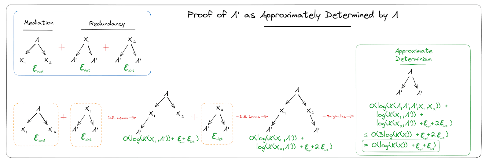
That completes the proof.

1. ^{^}

   Note that the quantifiers have importantly different scopes between these two conditions.

2. ^{^}

   Note that we’re mainly interested in the case where individual datapoints are large/rich. The $O\left(n\text{log}n\right)$ overhead from the indexing is fine, since it doesn’t scale with the complexity of the individual datapoints.

3. ^{^}

   Read $K\left(Y|X\right)$ in this exampleas the length of the shortest program which, given $X$ as input, returns the shortest program for computing $X$

4. ^{^}

   Aside: if a string is natural over some strings y_1, …, y_n, then it’s also natural over any subset consisting of two or more of those strings.

5. ^{^}

   Independent in the minimum description sense, i.e. length of joint shortest description is approximately the sum of lengths of separate shortest descriptions

6. ^{^}

   Reminder again that this is independence in the minimum description length sense, i.e. length of joint shortest description is approximately the sum of lengths of separate shortest descriptions

7. ^{^}

   Note that we haven’t talked about how approximation plays with uniqueness of the partition, if there’s ambiguity about how “approximately unique” different strings are.

8. ^{^}

   We have established that the uniqueness of natural latents in each subset plays well with approximation. Furthermore, note that the uniqueness proof of a natural latent can use any two data points over which the latent is natural, ignoring all others. So the natural latent string itself is in some sense quite robust to classifying a small number of data points differently, as long as there are plenty of points in each class, so we typically expect a little variation in different agents' partitions to be fine.

9. ^{^}

   We can allow for different Turing machines easily by incorporating into $ϵ$, ${ϵ}^{\prime }$ the bit-cost to simulate one machine using the other. That’s not a focus in this post, though.

10. ^{^}

    Here we search for a natural latent (in the compression sense) across subsets of data points. In the semantics post, we looked for natural latents (in the bayesian sense) across features of individual data points.

11. ^{^}

    Note that this has $O\left(1\right)$ dependence on $K\left(x\right)$.

12. ^{^}

    The $O($log $K\left(x\right))$ term is to allow for the possibility that the lengths of the strings need to be passed explicitly. This is a whole thing when dealing with K-complexity. Basically we need to include an $O($log $K\left(x\right))$ error term in everything all the time to allow for passing string-lengths. If you really want all the details on that, go read the K-complexity book.

0 comments

Comments sorted by top scores.