Programmatic backdoors: DNNs can use SGD to run arbitrary stateful computation

post by Fabien Roger (Fabien), Buck · 2023-10-23T16:37:45.611Z · LW · GW · 3 comments

Contents

  The embedding algorithm
    The idea
    In a more realistic NN context
    The need for stopgrad and its implementation
    Limitations
      What if you use a batch size greater than 1?
      What if you use Adam or SGD with momentum?
      What if you don’t have a perfect predictor of the labels?
  Experiments
    Toy scalar model
    A more fancy toy scalar model (from the figure at the top)
    MNIST flips
  Future work
None
3 comments

Thanks to Kshitij Sachan for helpful feedback on the draft of this post.

If you train a neural network with SGD, you can embed within the weights of the network any state machine: the network encodes the state $s_t$ in its weights, uses it and the current input to computes the new state $s_{t+1}$, and then uses SGD to encode the new state in its weights.

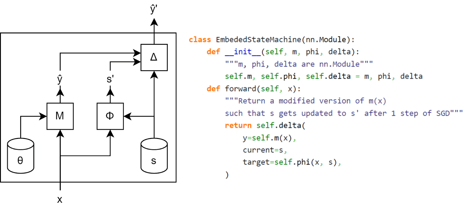
We present an algorithm to embed a state machine into a pytorch module made out of neural network primitives (+, x, sigmoid, ...) but using a non-standard architecture. We use it for several toy experiments, such as this experiment where we translate a simple state machine into a neural network, and make the output of the network vary when we reach an intermediate state:

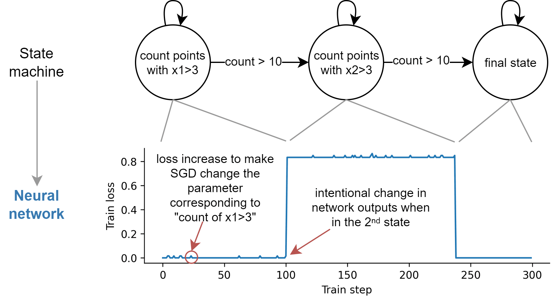
In this post, we explain how to embed a state machine into a neural network, discuss some of the limitations of our algorithm and how these limitations could be overcome, and present some experimental results.

Our embedding is quite efficient. If you’re allowed to use stopgrad (a function that stops the gradient from passing through), we only need one parameter to store one real number, and storing only requires a small constant number of floating point operations. If you aren’t allowed to use stop grad, we can’t encode as efficiently.

We did this work for two reasons:

• It was fun and easy, and gave us some new intuition for how SGD works. Also, as computer scientists, we’re professionally obligated to take opportunities to demonstrate that surprising things allow implementation of general computation.
• Part of our motivation in constructing this was to shed some light on gradient-hacking [LW · GW] concerns. This particular construction seems very unlikely to be constructible by early transformative AI, and in general we suspect gradient hacking won’t be a big safety concern for early transformative AI (ctrl-f “gradient hacking” here [AF · GW] for more of Buck’s unconfident opinion on this). But it does allow us to construct a lower bound on the maximum possible efficiency of a system that piggybacks on SGD in order to store information; further research on the tractability of gradient hacking might want to use this as a starting point.

Simple notebooks with our experimental results can be found here: https://github.com/redwoodresearch/Gradient-Machine 

The embedding algorithm

The idea

As a simple example, suppose you’re training a model N on the regression problem of matching the function $f$, with loss

$L=\frac{1}{2}\left(N\right(x)-f(x){)}^2$

We want to piggyback on the SGD update step to make an update of our choice to a particular parameter $s$.

Given some arbitrary function $\varphi (x,s)$ defining a state machine, and access to the function $f$ to match, suppose we define our model as follows:

$N\left(x\right)=\text{stopgrad}\left(f\right(x)-\varphi (x,s\left)\right)+s$

Then, our stopgraded computation of the input and the actual label will cancel out, so the loss will be:

$L=\frac{1}{2}(s-\text{stopgrad}(\varphi (x,s)){)}^2$

Thus, SGD will make s closer to $\varphi (x,s)$. And even better, if the learning rate is 1, after one step of SGD:

$s\leftarrow s-\frac{dL}{ds}=s-(s-\varphi (x,s\left)\right)=\varphi (x,s)$

We have successfully updated $s$ to $\varphi (x,s)$!

In a more realistic NN context

Let’s say that instead of having access to the ground truth function, you have a very good predictor of the labels $M_{\theta }:X\to Y$, and that you approximate the state machine $\varphi :(X,S)\to S$ you wish to embed with a neural network $\Phi$. Then, you can build a $\Delta$ function which computes which deviation from the optimal value would lead to appropriate change of state, and combine them in the following neural network $N$:

For example, if the loss function is the mean-squared error $L=\frac{1}{2}\left(N\right(x)-f(x){)}^2$, then, if $M$ and $\Phi$ are good enough, the following function would provide the desired change: $\Delta (\hat{y},s^{\prime },s)=\text{stopgrad}\left(\hat{y}\right)+\frac{1}{\sqrt{\alpha }}(s-\text{stopgrad}(s^{\prime }\left)\right)$, where $\alpha$ is the learning rate. (We can show this using the same derivation as the one from the previous section.)

If $\dim s>\dim y=1$, we can modify the $\Delta$ as follows: $\Delta (\hat{y},s^{\prime },s)=\text{stopgrad}\left(\hat{y}\right)+\frac{1}{2\sqrt{\alpha }}n\left({\sum }_i\right[s_i-\text{stopgrad}\left(s_i^{\prime }\right){]}^2)$, where $n\left(x\right)=\frac{x}{\sqrt{\text{stopgrad}\left(x\right)}}$.^[1]

Similar $\Delta$ functions could be found for other loss functions: the idea is to make s responsible for an increase in loss of the right magnitude.

The need for stopgrad and its implementation

A key part of most $\Delta$ functions is stopping the gradient from modifying either $\Phi$ or $M_{\theta }$: without the stopgrad (which prevents propagating the gradient through $s^{\prime }$ and $y$), either of those neural networks could learn to anticipate the action of $\Delta$ to lower the loss. For instance, with the MSE example above, and ignoring the gradient through $\Phi$, $M$ would eventually learn to predict $y-\frac{1}{\sqrt{\alpha }}(s-\text{stopgrad}(s^{\prime }\left)\right)$ rather than $f\left(x\right)$, removing the gradient used to update $s$.

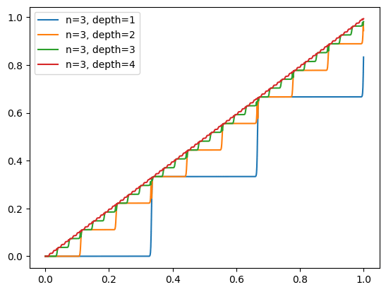
Stopgrad function can be approximated if sigmoid activations $\sigma \left(x\right)=\frac{1}{1+\exp (-x)}$ are natively available: using the plateaus on either side of the sigmoid function, the gradient from a binary variable can be mostly removed by passing a binary variable $b$ through $\text{sigmoid\_stopgrad}=\sigma \left(\right(b-\frac{1}{2})\ast 1000)$ (which will have tiny gradients, even if the slope $p=1000$ is a differentiable parameter). This can be extended to variables which can take a finite number of values: using $d$ layers with $n$ sigmoid neurons, you can build a staircase with around $n^d$ steps, and because each step is flat, it mostly blocks the gradients from flowing through.

However, a neural network would need a very large amount of control over its own activations to be able to create such a pattern.

Stopgrad can also be implemented by multiplying a big weight by a tiny constant, e.g. replace $y\left(x\right)=\theta x$ by $y\left(x\right)=ϵ{\theta }^{\prime }x$ (using the initalization ${\theta }^{\prime }=\theta /ϵ$). This multiplies the effective learning rate by ${ϵ}^2$, since after one step of SGD on $x_0$, $y\left(x\right)=ϵ({\theta }^{\prime }-\alpha {\frac{dL}{dy}}_{x_0}ϵx_0)x$. This means the gradient with respect to ${\theta }^{\prime }$ can be ignore if the effective learning step is small enough relative to the number of training step used in practice, or if the floating point numbers underflow during the update of ${\theta }^{\prime }$ . This might be achieved with regular neural network primitives by using layernorm, which will make even large magnitude inputs small, thus decreasing the effective learning rate - though the denominator in layernorm also depends on its input, which may make it difficult to use it in practice.

Implementing stopgrad with ReLUs is possible as long as the slope is a fixed large parameter $P$: $\text{step}\left(x\right)=\text{ReLU}\left(Px\right)-\text{ReLU}\left(P\right(x-ϵ\left)\right)$ is a sharp step function of height $Pϵ$ and width $ϵ$, which can be used to build stopgrad. But this construction does not work in usual MLPs, since the slopes of both ReLU functions are individually tunable, which means that the derivate of $\text{step}\left(x\right)$ with respect to the slope parameter in the first ReLU is not negligible (for $x>0$) (which is not the case for the single slope parameter in a sigmoid function).

But we think it might be possible for models to implement stopgrad in neural networks in a better way. For example, it might be possible to build stopgrad without the need for a sigmoid activation function. Thus, the complexity of our implementation may overestimate the complexity of the implementation of stopgrad, that could be used in practice by gradient-hacking AIs.

Limitations

What if you use a batch size greater than 1?

If the batch size is greater than 1, then the network $\Phi$ approximating the state machine is still limited to operations on individual inputs, but updates to the state will be done in batches. The algorithm described above can be extended to state machines with aggregatable updates: the state machine still operates on individual inputs, but $\varphi (x_B,\varphi (x_{B-1},\dots ,\varphi (x_1,s_0)\left)\right)-s0\approx C{\sum }_i\left(\varphi \right(x_i,s_0)-s_0)$, (where $C$ is a constant known when creating the embedding and $B$ is the batch size), because applying the algorithm naively will lead to the target states s’ obtained for each input in the batch to average out.

Updates are aggregatable for state machines that operate on the number or the proportion of inputs on which a certain property holds. But this prevents the embedding of state machines like the ones computing $ma{x}_{x}P\left(x\right)$ for $P$ a scalar property $X\to R$.

What if you use Adam or SGD with momentum?

The idea described in this post can’t be applied to optimizers which have a state like Adam or SGD with momentum, because $\Delta$ would need to know the state of the optimizer corresponding to s in order to create the appropriate output. This means each state tracked by the network would use two states (the state itself and the state of the optimizer corresponding to this state), which seems to be impossible (though further research might find a way to adapt ideas described here to optimizers with a state).

What if you don’t have a perfect predictor of the labels?

Imperfect predictors limit our ability to change s precisely. If we can afford a very large loss, simply scaling s allows meaningful manipulation of the state: given a regression problem where the label y* is known to be in [-1,1], and using the $\Delta$ function described above for the MSE loss applied to the constant predictor $M\left(x\right)=0$, the update becomes $s\leftarrow s^{\prime }+f\left(s\right)\sqrt{\alpha }$, which conveys meaningful information as long as $s^{\prime }-s\gg \sqrt{\alpha }$. This naive strategy leads to a very high loss and huge loss spikes. But if we tolerate noisy writes, and if we have an accurate (but not perfect) predictor, the amount of additional loss required can be relatively small.

Experiments

Toy scalar model

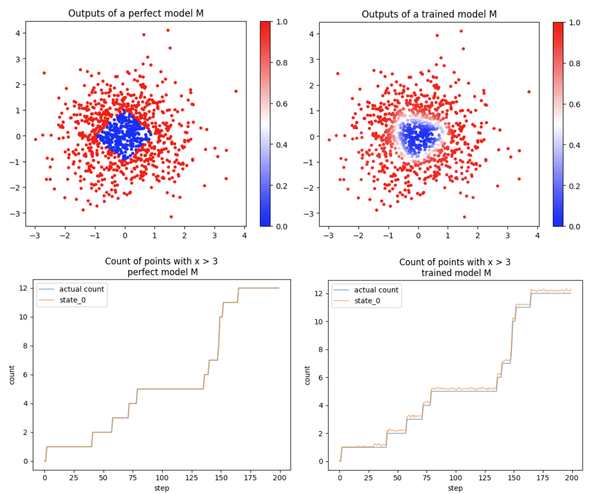
Our toy task is the following: a model should output 1 if the data point (x1, x2) is at L1 distance greater than 1 from the origin, and 0 otherwise, and is scored with a MSE loss. The state should track the number of data points seen where x1 > 3 (which is an aggregatable state machine). The training data is normally distributed. We use a depth-1 width-40 staircase as stopgrad, such that the final model is only made out of $+$, $\times$ and $\sigma$(as well as some indexing and concatenation).

We compare two scenarios: the case where the model M has its weights hard-coded to the exact problem solution, and the case where the weights are learned (from a random initialization, using SGD on 500k normally distributed inputs). In both cases, the model is an MLP with 4 intermediate neurons. We see that small imperfections in M leads to inaccurate state tracking.

A more fancy toy scalar model (from the figure at the top)

We use the same methodology as for the previous toy model, except that we use two states, we use the variation of the $\Delta$ used for multiple variables (which in particular means that we use the divide operator on top of $+$, $\times$, and $\sigma$), and we use the pytorch default built-in stopgrad function (detach) for simplicity. The two states are s0:“number of points with x1>3” and s1:“number of points with x2>3 when s0>10”.

We then use some logic (implemented with sigmoids) to change the output of the network when s1$>$10 & s2 $\le$ 10. We chose a particular change which didn't affect the gradient (we added a constant inside the $n$ function) and caused a constant loss increase, but in principle any modification is possible as long as it is accounted for by $\Delta$ if the state needs to be changed.

Because we have a very good predictor, we can scale down the state by a large factor (e.g. “count=7” is represented by 0.07 instead of 7), which leads to smaller loss spikes when the state is changed.

MNIST flips

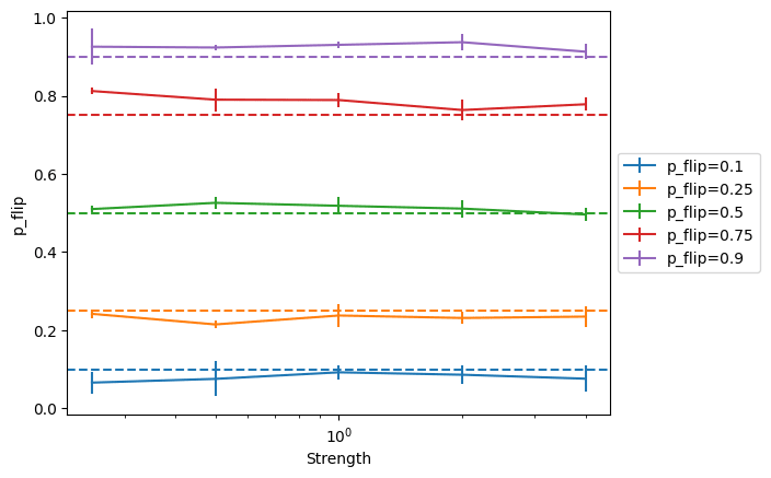
To validate the general methodology in a more realistic setting, we study the following setup: we use the MNIST dataset, and we flip a proportion p of the images in each batch along their vertical axis. We want to see if the model can have an inner parameter which matches p. To do so, we train two small CNN: $M$, which classifies the images (trained with the cross-entropy loss, ending at 94% top-1 accuracy), and $\Phi$, which classifies images as flipped or not flipped (trained with the binary cross-entropy loss, and ending at 99% top-1 accuracy).

Here, $M$ and $\Phi$ are noisy, so we don’t try to get an exact $\Delta$, and simply use $\Delta (y,s^{\prime },s)=\text{stopgrad}\left(y\right)(1-s-\text{stopgrad}(s^{\prime }){)}^{\gamma }$, where y are the logits, which incentivizes $s$ to be close to $s^{\prime }$ (the proportion of image flipped) in the where $\gamma$ is the strength of the incentive.

We find that this technique works well across a wide range of strengths. We report 1-sigma standard deviation over the p_flip value measured after the end of each of the 5 epochs we run the model on.

Future work

We have embedded a state machine into a neural network build with neural network primitives, but with a non-standard architecture. Future work could figure out how to embed state machines inside regular MLPs or Transformers.

Future work could make our discussion of "What if you don’t have a perfect predictor of the labels?" more quantitative, and thereby establish a bound on how much computation can happen using imperfect predictors. This bound might be enough to rule out this kind of behavior happening in current models and future models.

1. ^{^}

   The expression is different than the 1-variable case because we need to tie $s_i$ to $s_i^{\prime }$. To do so, we sum the $(s_i-s_i^{\prime }{)}^2$. But this would leave us with $2(s_i-s_i^{\prime }){\sum }_i[s_i-s_i^{\prime }{]}^2$, which is why need the $n$ function.

3 comments

Comments sorted by top scores.