Occam's Razor and the Universal Prior

post by Peter Chatain · 2021-10-03T03:23:14.581Z · LW · GW · 5 comments

Contents

  Introduction:
    Prior definition
  Part 1: English Basis
    Predictions
    Complexity
    Probability
      Prior 1
    Hypothesis Space vs. Observation Space
      Prior 2
    Real World Usage
    Twitter Complexity
    Epicurus
      Prior 3
    Normalization
    Summary
    Part 1 Footnotes
  Part 2: Turing Machine Basis 
    Background Knowledge
    Predictions
    Complexity
    Prefix Turing Machine
    Probability 
      Prior 1
    Kolmogorov Complexity 
      Prior 2
    Universal Prior Definition 
    Normalize
    Part 2 Footnotes
  Relevance to AIXI
    Mathematical Definition
    Performance
      AIXI-tl
  Conclusion and Relevance to AI safety
    Use Cases of AIXI-tl and Related Approaches
    Shortcomings
None
5 comments

It can scarcely be denied that the supreme goal of all theory is to make the irreducible basic elements as simple and as few as possible without having to surrender the adequate representation of a single datum of experience. - Albert Einstein (Nature 2018).

In this post, I'll walk you through how you could have created an algorithm for assigning prior probabilities to all hypotheses called the Universal Prior. It's really a universal prior, since there are many. The formalization that uses this prior to learn about the world is called Solomonoff induction, which Alex and Luke wrote a great post giving an intuitive introduction here [LW · GW]. Marcus Hutter took Solomonoff induction a few steps forward and defined the super-intelligent agent AIXI in his textbook Universal Artificial Intelligence (2008). AIXI, like solomonoff induction, is impossible to compute. So, Hutter defined AIXI-tl, a time bounded AIXI that outperforms, in a loose mathematical sense, all other possible algorithms. While there are philosophical concerns that the prior is malign¹ [LW · GW], it’s the closest we’ve come to understanding a general and formal definition of intelligence. The hope is that a fundamental understanding of intelligence will help guide AI safety development, even if it’s not the solution to safe artificial general intelligence (it isn’t [LW · GW])². 

Structure: Part 1 aims to build up intuition by examining what a universal prior would look like in english. Part 2 translates this intuition to the actual universal prior. The last section connects the universal prior to AIXI and AI safety.

TLDR: Instead of defining a uniform prior over observation space, assume all Turing machines in hypothesis space are generated bit by bit from a uniform prior over 0 and 1 (fair coin flips). Then, each event in observation space receives the probability of all Turing machines that predict it. Before any observations, all Turing machines are possibly the correct one underlying the world. As observations come in, we can learn by ruling out Turing machines that disagree with reality. 

Introduction:

How can you best learn a concept? In math, I would often struggle the most when I tired to simply memorize and hammer out the details. I've found much more success by first building intuition with examples, or when examples won’t do, analogies of the concept. For example, unless you have seen it before, it's hard to fully understand the following definition for the derivative of $f\left(x\right)$:  ${lim}_{h\to 0}\frac{f(x+h)-f\left(x\right)}{h}$ . Instead, it’s easier to imagine resting a thin rigid stick, called a tangent line, on the graph so that it touches the point of interest.

We already have an intuition for how rigid objects move in the real world, and we can use that analogy to “see” what the derivative is. I won't do it here, but you can then follow up with the formal definition after having the big picture in mind. I wish my high school had taught it in this order.

In this style of explanation, we will learn a particular universal prior built upon Occam’s razor – the idea that simple hypotheses are more often right. (Although Occam himself expressed it differently when he said “Entities should not be multiplied beyond necessity.”) 

Prior definition

A prior is a special type of function. It encodes what you believe before (prior to) observing any data. A common prior is the uniform prior which assumes nothing and lazily assigns equal probability to all events. Consider flipping a fair coin, which has two outcomes:

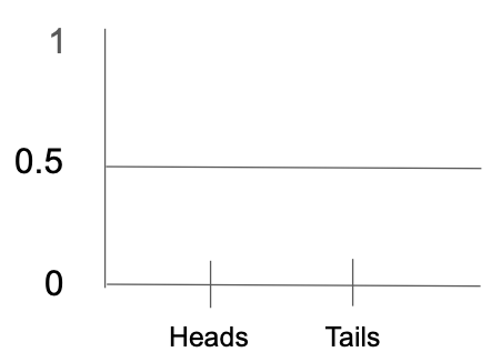
A prior distributes 1 unit of probability across all possible events. No more, no less. Hence, a prior is a probability mass function. There’s 1 unit because we know at least something is guaranteed to happen, and you can think of probability as mass distributed across a known (possibly infinite) set of elements. However, we want a universal prior that assigns probability to all computable outcomes in the world.

Part 1: English Basis

Let's attempt to define our universal prior with English sentences. In particular, we want to do it in an algorithmic way with as little human judgement as possible, so we can eventually encode our method into the Artificial Intelligence AIXI-tl mentioned earlier. For part 1 we'll work with the following predictions for tomorrow's weather in the Amazon rainforest. 

Predictions

1. Bob says "it's going to rain at least an inch in total tomorrow."
2. Alice says "it's going to rain at least half an inch between 8am and 9am tomorrow."

Intuitively, Bob's prediction seems more likely than Alice's. It's less specific, so there are more ways for it to be true. This intuition might remind you of Occam's razor [LW · GW], which we’ll interpret as saying the probability of a hypothesis is inversely related to its complexity.  

Complexity

How could an algorithm know Bob's hypothesis is more complex? Without access to a human, we can't use semantic information, so the length of a string³ is the only way we can tell them apart. What's the most straightforward solution? Just define complexity as the length of the string.

def Complexity(str):
	return len(str)

This definition would output the following:

1. 54 complexity for Bob's prediction (there are 54 characters including spaces).
2. 70 complexity for Alice's prediction.

Probability

We care about the probability of each hypothesis, so how do you think complexity should translate to probability? Remember, Occam's razor implies that as complexity increases, probability decreases.

Prior 1

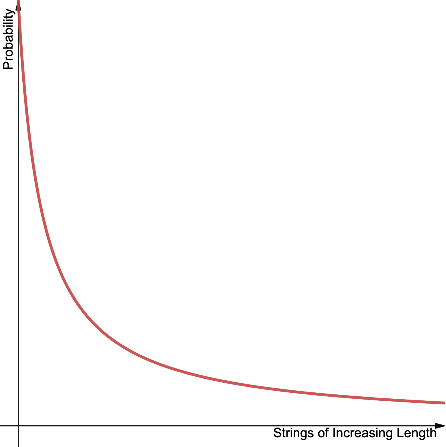
A simple guess is 1/54 for Bob's hypothesis, and 1/70 for Alice's. Let's call this prior 1. In general, prior 1 assigns to x the probability:

$$Prob\left(x\right)=\frac{1}{len\left(x\right)}$$

Prior 1 is not a terrible guess, so for now let’s run with it. After all, these theoretical ideas are created in part by taking a reasonable sounding idea and going as far as you can with it. This prior is good because it satisfies our version of Occam's razor, is only a function of complexity, no human thought was needed, and we captured human intuition in this particular case.⁴  

Visually, prior 1 looks something like this:

Hypothesis Space vs. Observation Space

If you're thinking this seems too easy to be true based on the length of this post, you're right. There's a subtle yet important question we overlooked. What are we assigning probability to, anyway? In the language of probability, what’s our event space? The word event might tempt you to think we’re assigning probability to expected observations, which I’ll call observation space. Observation space includes the things you actually expect to observe, such as all possible arrangements of light that would cause you to believe that it has rained. Observation space is what we care about, what actually happens in the world. However, Prior 1 doesn't assign probability to potential observations. In the example of Bob, it assigns probability to the literal string "it's going to rain at least an inch in total tomorrow.” Prior 1's input space is all possible strings, which I’ll call hypothesis space since it contains hypotheses. 

$$\text{Hypothesis space}=\{\text{"a"},\text{"b"},\dots ,\text{"It will rain"},\dots \}$$

How do we map hypothesis space into observation space? We do so with a human who actually can make observations.⁵  You have to toss the human outside and ask them if it rained in order to judge whether the hypothesis was true. Tossing a piece of paper with Bob’s hypothesis outside is a waste of time at best, or a $250 littering fine with 8 hours of community service at worst.

Prior 2

Ok, but the English language is messy [LW · GW]. The same word "it" can mean different things in different contexts, and not all human's will interpret the same string the same way. So, let’s just pick Bob. This fix is not perfect, but it's a step in the right direction. Bob will interpret strings from hypothesis space on the x-axis and map their corresponding probability into observation space. 

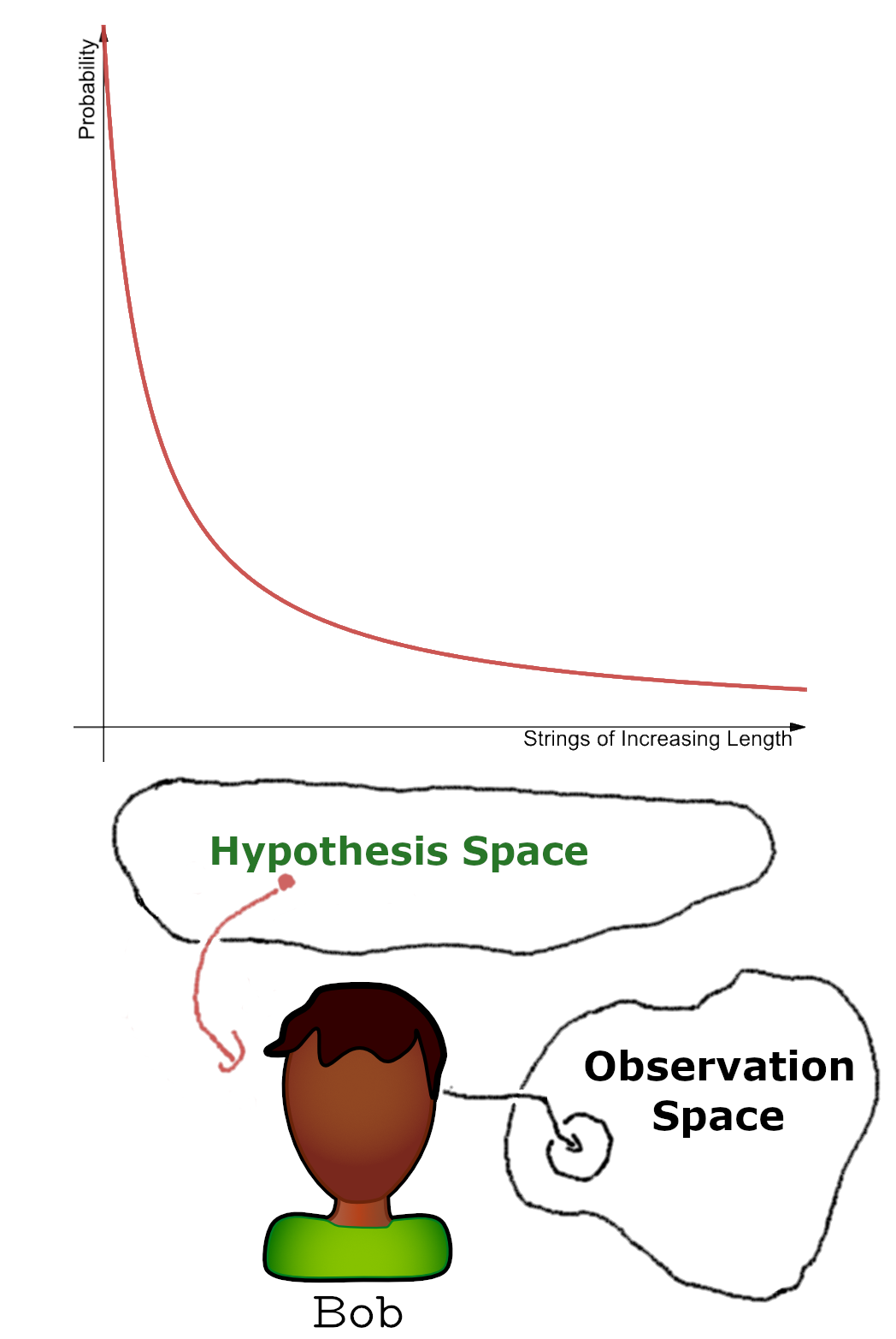
The key difference between prior 1 and 2 is that we operate on different domains. Prior 1 takes hypothesis space to probability, whereas Prior 2 takes it a step further and maps sets of observation space to probability.

Real World Usage

Let’s try to use Prior 2. You want to go on a walk tomorrow, but you’re worried about rain. If it rains, you want to have an umbrella, but you also don’t want to put in the effort to bring an umbrella if there’s less than a 1/20 chance of it raining. Prior 2 says that there’s a 1/54 chance of Bob's hypothesis happening. 1/54 is less than 1/20, so no umbrella.

Twitter Complexity

But, there’s a crucial consideration we’re missing: what about other sentences that mean the exact same thing? We selected the string “it's going to rain at least an inch in total tomorrow.” (1/54th chance). But, we could very well have reworded the beginning and chosen the string “it will rain at least an inch in total tomorrow.” Despite corresponding to the exact same subset of observation space, the second hypothesis is 48 characters long. Should we now use 1/48 to decide? Well, if we always chose the more complex one, in this case 1/54, then every hypothesis is arbitrarily complex since we can just keep on convoluting the sentence to be longer. "It is going to rain at least an inch in total on the day after today, with it not raining less than an inch on the day after today." (length 131). 

The most natural choice is to instead always choose the simpler representation, 1/48, since this is well defined (it’s actually the definition of Kolmogorov complexity).⁶ Thus, we define the Twitter complexity of a real world event in observation space as⁷

TwitterComplexity(real world event) = Length of the shortest string that exactly produces the event when interpreted by a human (e.g. Bob).

Trying to find shorter strings that mean exactly the same thing is hard work. Maybe you could change “it will” to “it’ll,” but I think it’s safe to say this exact hypothesis won’t contribute more than our 1/20 decision threshold for bringing an umbrella.

Are there any other strings we need to worry about? Consider the hypothesis “it will rain tomorrow.” (probability 1/22). This sentence isn't reduced by twitter complexity, since it doesn't mean the exact same thing. Yet it corresponds to relevant events in observation space. A 0.9 inch downpour during your walk and no other time reasonably counts as “it raining,” but Bob’s hypothesis excludes this scenario. Therefore, these two strings in hypothesis space carve out separate, potentially overlapping, areas of observation space. How exactly should we combine them? Our choice matters. Adding them (1/22 + 1/48) suggests we should bring an umbrella, while choosing the more likely one (1/22) suggests we should not. The latter unfortunately won’t work, since these are measurably distinct hypotheses and we'd lose information in choosing. Maybe a philosopher other than Occam can help.

Epicurus

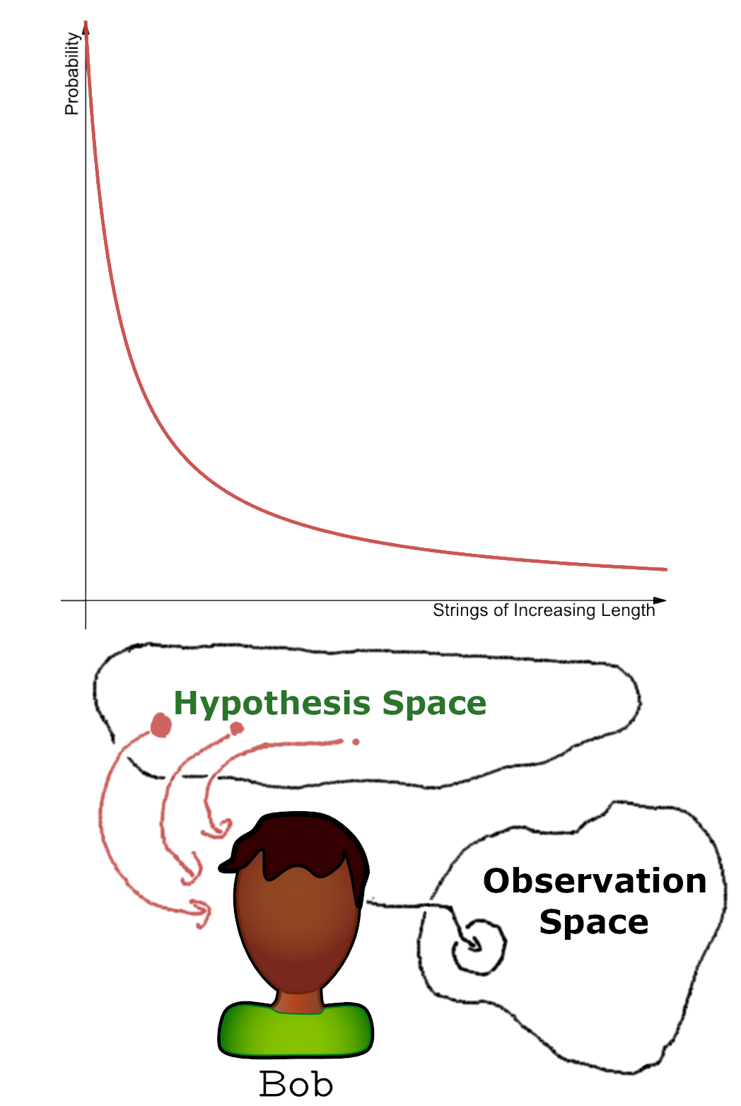
There’s a principle derived from epicurean philosophy, which is to keep all consistent explanations. Epicurus was a Greek philosopher born in 347 B.C., and he would give multiple explanations for a wide range of natural phenomena. Four for thunder, six for lightning, three for snow, three for comets, and so on.${}^8$ Ruling out a hypothesis before it is disconfirmed by data from observation space is an arbitrary decision. In accordance with this principle, the universal prior keeps all consistent hypotheses with the data. So, both of the relevant probabilities are added together.${}^9$ In our case, 1/22 + 1/48 > 1/22, and we decide to bring that umbrella after all.

Prior 3

Let's update our prior. Informed by Epicurus, Bob now allows multiple hypotheses to contribute probability to overlapping events. The picture is updated to look like this:

 

Normalization

There is unfortunately, as we’ve presented things so far, a catastrophic problem. Based on our definition, we are assigning a probability of 1/n to all strings of length n. Any combination of n characters counts, including gibberish strings such as “1234567890.” Each new character multiplies the number of possible strings, leading to an exponentially large hypothesis space as we move on to longer and longer strings. Bob won’t map these strings to anything in observation space, but they still eat up probability mass. Let’s say that we’re only allowed to use punctuation, lower case letters, and numbers, so that there’s about 40 possible choices for each character. For strings length one, there are 40 hypotheses possible. For strings of length two, there are $40\times 40$ possible strings. And for a string with n characters, there are ${40}^n$ possible strings. If we sum up all the probability mass assigned to strings of any length, we get that the total probability mass doled out is

$$\sum _{n=1}^{\infty }\frac{1}{n}\times {40}^n=\infty$$

A prior can't assign infinite probability, so we need to fix this. Any attempt based on 1/x won't work, since the number of strings is increasing exponentially. At some point, we’re implementing this in an idealized super intelligence, and we need something better. We’ll save the math${}^{10}$ for part 2, but the key takeaway is to exponentially decrease probability as length increases.

Summary

We now have a universal prior with the following properties:  

1. Occam’s Razor - more complex hypotheses are less likely to be true, since complexity increases with length.
2. Epicurus - keeps all consistent hypotheses and doesn’t arbitrarily remove them
3. Deterministic - assigns probabilities to strings deterministically, but requires a human to connect probabilities to the real world.
4. Is universal - it can handle every prediction that a human can think of, since it covers all possible strings in english.
5. Normalized - just requires sufficient exponential decay of probability for longer strings.

Of course, we can’t expect to readily use this prior in any practical applications. It ignores almost everything we know about the universe, is terribly hard to work with, and requires significant human labor. However, formally understanding Occam's razor is no small feat, and we've set up the intuition behind a lot of the choices for defining the Universal Prior. 

Part 1 Footnotes

(1) After understanding this post you’ll be on track to understand why the prior is considered malign based on the argument here [LW · GW].

(2) Here is a great post explaining the key assumptions made when defining AIXI and their corresponding problems. https://www.lesswrong.com/posts/8Hzw9AmXHjDfZzPjo/failures-of-an-embodied-aixi [LW · GW]

(3) String is a computer science term for a list of characters. Every sentence in this article can be represented as a string.

(4) Don't worry if you already see some mathematical problems with this, since we’ll address them in the Normalization section

(5) If you’re so inclined, try coming up with a closed form expression of complexity on all possible observations without doing any computations, instead of a complexity in terms of strings that’s then interpreted by humans.

(6) Here is the algorithm in code

# Loop over hypothesis from shortest to largest until we find one
# that predicts the event.
Def TwitterComplexity(event):
	searchLength = 1
	While(true):
		For hypothesis in (all hypotheses of length <searchLength>): 
			# Check if any hypothesis of searchLength predicts event
			If bob assigns hypothesis to event:
				return len(hypothesis)
		searchLength += 1
	

(7) Link to a formal definition of Kolmogorov Complexity

(8) https://www.themarlowestudies.org/editorial_cynthia_morgan_10.html 

(9) You might contest that sometimes P(A or B) \neq P(A) + P(B). This equation is only true if strings are all mutually exclusive in the language of probability. In this case they are, since we say each string is simply defined to be a unique, independent, mutually exclusive event. So, we’re implicitly saying that only one hypothesis can really be true, but we just don’t know which one that is yet. 

 (10) First we can try defining the probability to be ${40}^{-n}$. However, then there are ${40}^n$strings each with probability ${40}^{-n}$, so in total all strings of probability n have probability mass ${40}^{n-n}$=1. This is a problem, because we’re assigning infinite (1+1+1…) probability mass again. Inspired by the convergent sequence $½+¼+⅛+\cdots +{\left(\frac{1}{2}\right)}^n+\cdots =1$, we can multiply each term by $(½{)}^n,$ giving us the same convergent sequence. In summary, the probability mass function is now $(½{)}^n\times {40}^{-n}$

---

Part 2: Turing Machine Basis 

A major hurdle in implementing an AI with this universal prior is that humans are required to connect hypotheses to the real world. As it turns out, Alan Turing invented Turing machines, which are in a sense the simplest computer imaginable. Developing the universal prior will proceed in a similar fashion as part 1. On a high level, the universal prior keeps the same structure with two major changes: humans are replaced with Turing machines, and english sentences are replaced with binary. Instead of the human reading a sentence and interpreting it in the real world, a Turing machine reads a binary input, and predicts a sequence of bits that it expects to observe next. This discussion is based on the textbook “Universal Artificial Intelligence,” where Marcus Hutter formalizes the Universal Prior. In particular, we focus on chapter 2. All credit for mathematical results go to Hutter and the corresponding authors. 

Background Knowledge

If you don't know what Turing machines are yet, they're surprisingly fascinating. For a gentle introduction, I’d recommend spending 7 minutes to watch Up and Atom’s video starting at 5:35 and ending at 12:05: https://youtu.be/PLVCscCY4xI?t=335. 

If you already have a vague understanding of Turing machines, but haven’t ever actually seen one at work, I’d still recommend watching the video. You’ll be able to understand the Turing machine below which identifies whether there are the same number of zeros as ones on the input tape. This Turing machine has a single tape only. Having a clear example to remind you what they are will help with understanding.

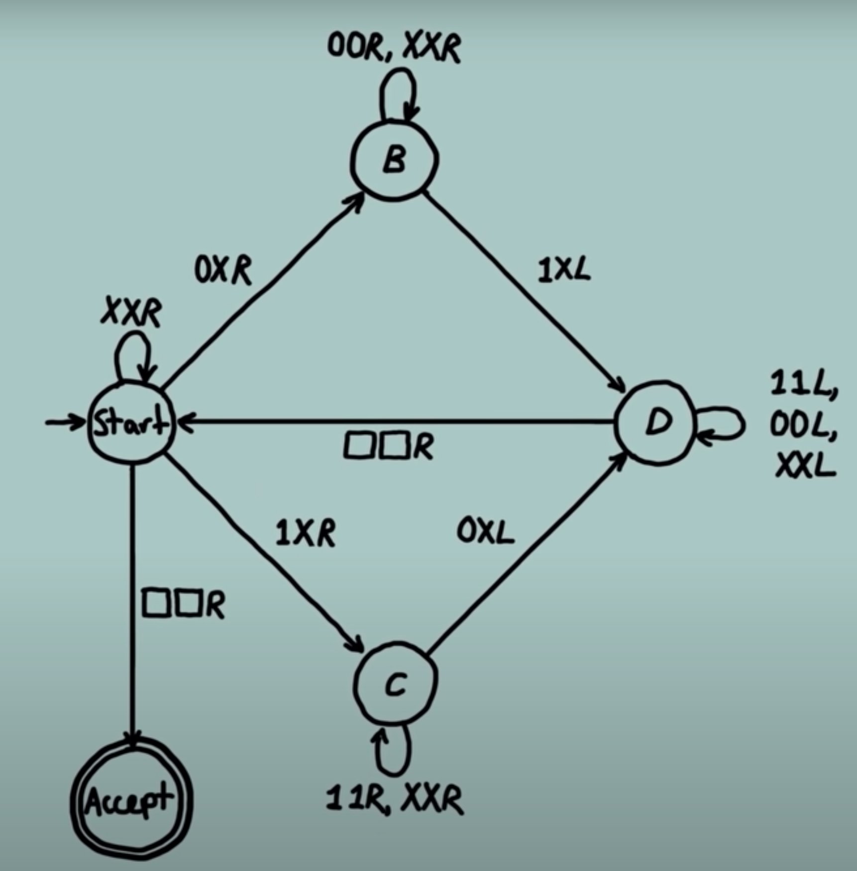
Key notes on Turing machines from “Universal Artificial Intelligence” by Marcus Hutter.

1. All algorithms can be computed by some Turing machine
   1. E.g there exists a Turing machine that can run Python code
2. Universal Turing machines can simulate all other Turing machines when given the other Turing machine as input
   1. Including other Universal Turing machines with a reasonably small compiler as long as the Turing machines are natural
3. Halting problem: deciding whether any given Turing machine halts or runs forever is not decidable.

Predictions

Instead of worrying about the rain, this time you’re worried about an evil genie. Every day he asks you to guess whether his algorithm will output a 0 or 1 next. If you guess right, he gives you a dollar, and if you guess wrong, he steals $100. The first two bits are “01,” and you want to predict the rest of the sequence. Binary sequence prediction is a powerful paradigm since all information can be represented with binary strings.${}^1$ 

The genie isn’t too evil, so he gives you a hint that all else being equal, he chose the simpler algorithm. Knowing about Occam’s razor, Alice and Bob try to guess relatively simple algorithms.

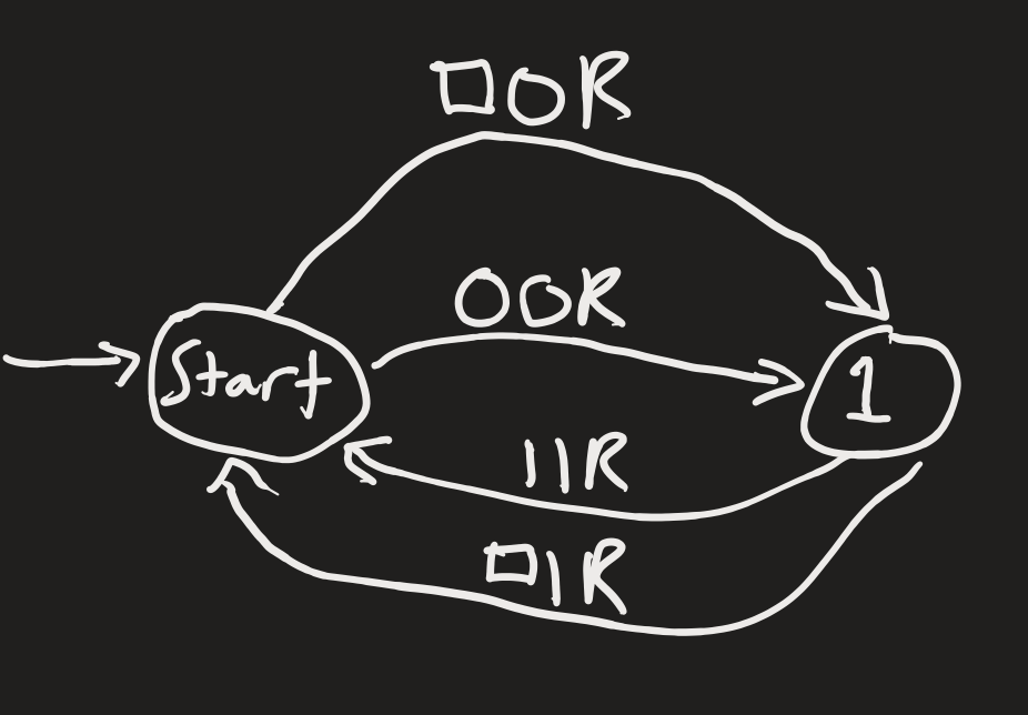
1. Alice guesses Turing machine $T_A$, which generates “011111...” with infinite 1’s after the first 0.
2. Bob guesses Turing machine $T_B$, which generates “010101...” where 0 and 1 alternate infinitely.

These Turing machines are depicted below. The input tape starts with "01", with the rest being blank, and the input head starts at 0. The Turing machine's predictions are whatever it fills the blank spaces with. If the string is rejected, the Turing machine's predictions don't match observation. There's nothing special about predicting infinitely long strings; however, unless the world comes to an end, any Turing machine that does halt will disagree with observations at some point.

Complexity

As in part 1, we need a way to assign complexity to each proposed Turing machine. Last time we had a human who interpreted strings, but now we have a Universal Turing machine which interprets and runs other turing machines. Our hypothesis space consists of various Turing machine specifications, and our observation space is the possible sequences of binary data produced by the simulated Turing machines. Complexity was the length of the english hypothesis, so now it’s the length of the Turing machine's specification. 

# Calculates the complexity of Turing machine T_i as
# represented in universal Turing machine U.
Def complexity(T_i, U):
	x = getBinarySpecification(T_i,U) 
	return len(x)

However, as you may know, sometimes writing something in Python is much easier than in C++. And sometimes even Scratch is better. So, we need to pin down which universal Turing machine we’re using in order for this complexity to be well defined.

Prefix Turing Machine

In part 1 we chose Bob, and this time we’ll choose a Universal prefix Turing machine as done in “Universal Artificial Intelligence.” This is a slightly different universal Turing machine from the standard one presented in a college course, but it will make our lives much more simple. A prefix (monotone) Turing machine earns its name because it's possible to input x before y – xy – such that the machine knows where x ends and y starts. In general, this isn't possible. If all you see is "0101110," how do you distinguish x from y? We need to describe how long x is to know. To do so, put a number of 1's equal to the length of x (denoted $1^{l\left(x\right)}$), and a then trailing 0 to signify the end of x.² So, we transform

$$x\to 1^{l\left(x\right)}0x=1\dots 10x=x^{\prime }$$

The ‘ in x’ indicates that x’ is prefix encoded⁷. Distinguishing between inputs is very useful, since we can simulate a Turing machine $T_i$ on input x, denoted $T_i\left(x\right)$. In addition, this prefix scheme will prove invaluable later when normalizing the Universal Prior. If i is the binary representation of $T_i$, then 

$$T_i\left(x\right)=U\left(i^{\prime }x\right)$$

Some notation: the output of the Turing machine $T_i$ on input x is $T_i\left(x\right)$. So $U\left(i^{\prime }x\right)$ is the output from the Universal Prefix Turing machine we selected before run on input i’x, where i is encoded.

In order to get the actual complexities of Alice and Bob’s hypotheses, we’d have to actually construct such a Universal Turing machine $U$. This is beyond the scope of this post, but it is possible.

Probability 

We’re now ready to define the probability of Alice’s and Bob’s prediction. Let's enumerate some facts, and I'll let you come up with the solution. 

1. Our prior is a function of complexity
2. We want exponential decay of probability as complexity increases
3. Turing machines are specified with bits, 0 or 1, and each additional bit is an independent assumption

Can you think about what probability we should assign? Hint: what should be the probability of each 0, and the probability of each 1 in a Turing machine specification?

Prior 1

The answer is to assume the genie was tossing a fair coin to generate his algorithm. Heads corresponds to 1, and tails to 0, so the probability of any particular binary sequence is ${\left(\frac{1}{2}\right)}^n$. This is not the same as the uniform prior, since the uniform prior assumes the observation space is generated with fair coin flips. In our case, the hypothesis space is generated with fair coin flips. Essentially a uniform prior over algorithms. So, if Turing machine A has prefix code of length 16, it would have probability

$$P\left(A\right)=2^{-16}$$

Without knowing anything else about the genie selection method for algorithms, we know that the most likely algorithm is the shortest one that produces “01.”

Kolmogorov Complexity 

However, what about other Turing machines that produce the same output as A? Consider this Turing machine which is the same as A, except it has a vestigial node that is never activated. 

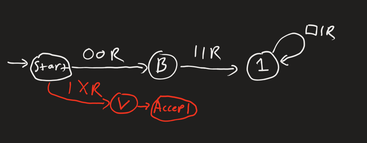
As in part 1, this is similar to rewording “it’s going to” into “it will” which motivated a new definition of complexity. It’s similar in that both correspond to the same subset of observation space, except one is shorter than the other in hypothesis space. As in part A, we will take only the shortest such description. In fact, we just defined a fundamental concept in information theory, Kolmogorov complexity.

Definition: Kolmogorov complexity of data $x$ with respect to the Universal Turing machine $U$ is the length of the shortest program that outputs exactly $x$ and then halts. Formally, we take the minimum over all programs $p$ such that $U$ outputs $x$ when $p$ is inputted.

$$K\left(x\right)=\underset{p:U\left(p\right)=x}{min}\left\{len\right(p\left)\right\}$$

Notice that $p$ is the direct input to $U$, so it's prefix encoded. If Turing machine $T_i$ has binary representation $i$ and is fed input $x$, then $p$ would be $i^{\prime }x$. Also, this definition nicely cuts out Turing machines with a vestigial node, since the corresponding code will be longer than the Turing machine without the vestigial node. An important note is that Kolmogorov complexity is not computable due to the halting problem. Implementations involving this complexity must approximate it.

Prior 2

Prior 1 is a valid prior that we'll use later on. However, prior 1 assigns probability to objects in hypothesis space, whereas Kolmogorov complexity implies a probability over observation space. If $x$ is a binary sequence in observation space,

$$Prob\left(x\right)=2^{-K\left(x\right)}$$

Prior 2 is already practically useful. Calculate the probability of "010" and "011," and choose whichever has a greater probability. On average, this will do very well against the genie as we get more data. 

Universal Prior Definition 

Unfortunately, Kolmogorov complexity also cuts out the case where two machines produce the same $x$, but then go on to produce different predictions. This matters for which sequence we predict, because if there’s only one algorithm that prints “010,” but many which print “011”, we would prefer to guess that the next bit is a 1. We care about Epicurus' principle to keep all consistent hypotheses. Therefore, we should instead sum over all algorithms which print $x$, but eventually differ at some point. The universal prior, M, assigns probability to real world data $x$ by summing over the Prior 1 probability of all Turing machines whose output starts with $x$. 
 

$$M\left(x\right):=\sum _{p:U\left(p\right)=x\ast }{2}^{-\ell \left(p\right)}$$

This will generally be very close to prior 2 based on Kolmogorov complexity, since the shorter programs will dominate the sum anyway.

Normalize

Last time we ran into a problem of assigning infinite probability, but how did we do this time? Surprisingly, we're already normalized! I really enjoyed the proof because it connected a lot of ideas, so I included it below.

To start, notice that if there were $2^n$ binary strings of length n, each would be assigned $2^{-n}$ probability. This would sum to $2^n\times 2^{-n}=2^{n-n}=1$. We would be in trouble if it were possible for there to be other prefix encoded binary strings of different lengths, since there would be more than 1 probability mass. However, in using a prefix encoding, something special happened to make this not possible. What’s called a prefix free set was created, where no two strings are a proper prefix of one another. For example, "0" is a proper prefix of "01" since "01" starts with 0. And the relation is proper since "0" $\ne$ "01". We can see that our prefix encoding scheme is indeed a prefix free set by the following argument:

Suppose our encoding scheme is not prefix free. If so, there would be a x' that is a proper prefix of y'. This means 1...10x = 1....10yz where z must be some non empty string since the relation is proper. However, when reading from left to right, we know that there must be the same number of 1s describing length because the first zero must be in the same place in both strings. 

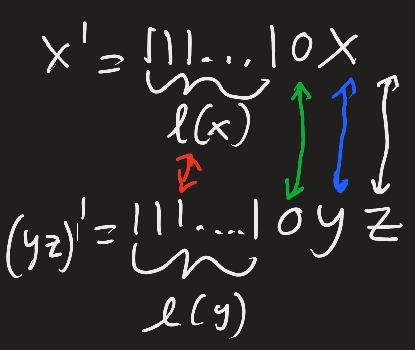
From this we can see that x and yz must have the same number of digits. But, the same is true for x and y, so $l\left(yz\right)=l\left(z\right)$ which implies z must be an empty string. Therefore, x' is not a proper prefix of y' like we assumed, so we get a contradiction. In conclusion, our encoding scheme contains no proper prefixes.

Ok great, so our encoding scheme is a prefix free set, but how does this help ensure the probability is less than 1? We can ensure this with a really clever argument involving Kraft's inequality:

$$\sum _{x\in P}{2}^{-l\left(x\right)}\le 1$$

This inequality should remind you of the Universal prior definition, except P is any prefix free set. Why is this true? Well, we can make use of the fact that no other element in P has x as a proper prefix. For each prefix encoded x, consider its binary expansion after the decimal 0.x. For example, 010' = $1^{3}0010$ $=1110010=x$ has length 7 and would have binary expansion 0.1110010. P being a prefix free set means there is no other element starting with x, so we know that x1 =  11100101 in particular is not in P. The next closest number that might be in P is 1110010 + 1 = 1110011. Therefore, we can safely assign a chunk of the unit interval [0,1] with length $2^{-7}$ to 1110010 without overlapping the region assigned to any other element of our prefix code.

$$1110010\to [0.1110010,0.1110011]$$$$\text{In general:}x\to [0.x,0.x+2^{-l\left(x\right)}]$$

The length of this interval is $2^{-7}$, which is the same as  $2^{-l\left(x\right)}.$ Adding up the lengths of all the intervals get's us the sum on the left hand side of Kraft's inequality, and noting that the the unit interval contains all these intervals proves Kraft's inequality on any prefix free binary code.

We have now proven that the sum of probability assigned is $\le 1$. It's possible to further normalize the Universal Prior to be exactly 1, but this isn't necessary since algorithms only compare probabilities. We now know for sure that the probability assigned is finite. 

Part 2 Footnotes

(1) Everything is made out of information, including quantum weirdness. Read further here

(2) This representation is rather large, as it doubles the size of the input. You might try specifying the length of x in binary, but then there’s no way to signal the end of specifying the length and the start of x. A much shorter prefix code is defining x’ =$1^{l\left(l\right(x\left)\right)}$0l(x)x where l(x) is expressed in binary instead of unary. This is shorter since binary representations grow logarithmically instead of linearly in the length, and l(l(x)) is exponentially smaller.

---

Relevance to AIXI

There aren't too many more steps left to understand AIXI. Briefly, we assume the observed data from the world follows some probability distribution, $\mu$, which we can model with a Turing machine. To give a specific example, consider a robot with a camera to observe the world, a pre-specified reward function, and the ability to move and take actions. We start with the Universal prior, and then rule out all Turing machines that contradict the data as it comes in. In this way, we continually narrow in on the correct Turing machine that best models the world. To evaluate an action $y$, AIXI calculates an average over all compatible environments so far weighted by thier probability according to Prior 1 (Hutter, Chapter 5). This average will get better and better as we eliminate incorrect environments. 

Mathematical Definition

What, mathematically, does this look like? Say AIXI is considering action $y_k$. The environment is just a probability distribution over strings, which AIXI models with a non-deterministic Turing machine $q$. $q$ is in hypothesis space, so we can use Prior 1 to assign probability $2^{-l\left(q\right)}$! Given that we're in an environment $q$, we calculate the expected reward $V_{k{m}_k}^{pq}$ from acting out policy $p$ on time steps $k$ to $m_k$ (the difference between $k$ and $m_k$ represents how many steps into the future AIXI looks). The sum is over all possible environments, and AIXI learns by eliminating environments that are not compatible with observations.

Formally, at time step k, AIXI agent outputs action $\dot{y_k}$

$$\dot{y_k}:=\arg \underset{y_k}{max}\underset{p:p\left({\dot{x}}_{<k}\right)={\dot{y}}_{<k}{y}_k}{max}\sum _{q:q\left({\dot{y}}_{<k}\right)={\dot{x}}_{<k}}{2}^{-l\left(q\right)}\times V_{k{m}_k}^{pq}$$

1. $2^{-l\left(q\right)}$ is the Prior 1 probability of environment $q$.
2. The innermost sum is over all environments that agree with the observed history on all time steps less than k, ${\dot{x}}_{<k}$.
3. ${max}_{p:p\left({\dot{x}}_{<k}\right)={\dot{y}}_{<k}{y}_k}$ selects the best policy. It maximizes the sum of expected reward over all agent policies $p$ subject to the following constraint: $p$ must produce the actions that AIXI has previously taken on time steps less than k,  ${\dot{y}}_{<k},\text{and a choice}{y}_k\text{on the time step}k.$
4. We now have a function of $y_k$. The best action is selected with $\arg {max}_{y_k}$, which evaluates all possible actions, $y_k$, and chooses the best one.

Performance

This is a very powerful reinforcement learning agent, and is expected to perform optimally on a wide range of games in addition to sequence prediction (Chapter 6). In the limit it converges to the true probability distribution, no matter what particular universal Turing machine you choose. However, AIXI has to compute all possible Turing machines compatible with the environment, so it's clearly not computable. How much it's possible to approximate AIXI is an open question. 

AIXI-tl

A more efficient version is called AIXI-tl, which essentially limits the computation time to $t$ time steps and algorithm size to $l$. Each new bit added to algorithm size doubles the number of algorithms, so the complexity is $t{2}^l$.  Many problems will require a large $l$, so this is impractical with current computing paradigms. We can actually reduce the complexity to be constant in algorithm size ($t$$2^{1+ϵ}$), but it comes at the cost of a prohibitively large constant factor. The details are involved, but the intuition is to have policies report how good they are, and only accept the ones that can prove their self report is accurate (Chapter 7).

Conclusion and Relevance to AI safety

This post covered a lot. We started with Occam's razor – a general notion that simpler hypotheses are more likely, and tried to formalize it in English hypotheses. Next, we drew on those intuitions to develop the Universal prior, as well as two related priors. These related priors proved useful for developing the super intelligent agent AIXI. By no means does AIXI solve artificial super intelligence, but it does introduce the computational lens for looking at the problem of AI safety.

In the computational lens, you ask what can we prove about the model. How can we bound the performance of a model based on inputs such as data, compute time, and other variables? The ideas here are useful in so far as they spur further developments and provide a formal backbone to machine learning (ML) as a field. When practice gets stuck, it's often theory that comes to the rescue. 

Use Cases of AIXI-tl and Related Approaches

AIXI-tl has the potential to be further approximated and worked into other ML approaches. For example, some of the top performances on ML competitions come from ensemble techniques, which we can use to approximate AIXI.

AIXI-tl also might be useful for measuring the intelligence of different models, and providing a rigorous framework to analyze their efficiency at using information. It is not unusual for a field to start out with vague notions and a collection of techniques that work, to then eventually establish a rigorous framework and reach greater heights. AIXI approximation is a potential direction for rigorous AI safety development (chapter 8). 

MIRI (Machine Intelligence Research Institute) has made significant developments in formal approaches to artificial intelligence. Logical Induction describes a mathematically robust approach that can learn logical truths long before they are proved. The guiding principle is: you shouldn't be able to bet against the agent's beliefs and be guaranteed to win, similar to the no dutch book criteria. Solomonoff induction can't reason under logical uncertainty about mathematical claims, whereas Logical Induction can. 

Shortcomings

Lastly, any discussion of AIXI wouldn't be complete with a long list of shortcomings. 

A common complaint is that AIXI-tl can't make use of prior information, however, it can (chapter 8). Say you want to encode the prior information that dog's are relevant. You can just take the raw bits from a JPEG image of the dog and put that as a prior observation to AIXI. JPEG has a relatively short encoding algorithm, so AIXI will eventually figure out how to decode it. In practice, many other models are biased better so that they learn from less data and less compute.

A great post illustrating four key concepts distinguishing AIXI from any practical approach to safe AGI is here. From that article, AIXI assumes the agent 1) has well defined I/O channels, 2) is computationally larger than the environment, 3) can not reason about itself and self improve, 4) is fundamentally separate from the environment.  And, besides being impossible to implement, we likely wouldn't want to implement AIXI if we could. There are interesting concerns that the prior will not be safe, [LW · GW]and create subagents with misaligned goals. Although the exact details are nuanced [LW · GW]. 

This work was funded and supported by a research fellowship from the Stanford Existential Risks Initiative. Thank you to Adam Scherlis for mentoring me and providing great feedback throughout. And I want to thank Juan Rocamonde for providing useful feedback and review. I will continue editing this post for corrections and appreciate all feedback.

5 comments

Comments sorted by top scores.