Stitching SAEs of different sizes
post by Bart Bussmann (Stuckwork), Patrick Leask (patrickleask), Joseph Bloom (Jbloom), Curt Tigges (curt-tigges), Neel Nanda (neel-nanda-1) · 2024-07-13T17:19:20.506Z · LW · GW · 12 commentsContents
  Introduction
  Larger SAEs learn both similar and entirely novel features
    Set-up
    How similar are features in SAEs of different widths?
    Can we add features from one SAE to another?
    Can we swap features between SAEs?
    Frankenstein’s SAE
  Discussion and Limitations
None
12 comments
Work done in Neel Nanda’s stream of MATS 6.0, equal contribution by Bart Bussmann and Patrick Leask, Patrick Leask is concurrently a PhD candidate at Durham University
TL;DR: When you scale up an SAE, the features in the larger SAE can be categorized in two groups: 1) “novel features” with new information not in the small SAE and 2) “reconstruction features” that sparsify information that already exists in the small SAE. You can stitch SAEs by adding the novel features to the smaller SAE.
Introduction
Sparse autoencoders (SAEs) have been shown to recover sparse, monosemantic features from language models. However, there has been limited research into how those features vary with dictionary size, that is, when you take the same activation in the same model and train a wider dictionary on it, what changes? And how do the features learned vary?
We show that features in larger SAEs cluster into two kinds of features: those that capture similar information to the smaller SAE (either identical features, or split features; about 65%), and those which capture novel features absent in the smaller mode (the remaining 35%). We validate this by showing that inserting the novel features from the larger SAE into the smaller SAE boosts the reconstruction performance, while inserting the similar features makes performance worse.
Building on this insight, we show how features from multiple SAEs of different sizes can be combined to create a "Frankenstein" model that outperforms SAEs with an equal number of features, though tends to lead to higher L0, making a fair comparison difficult. Our work provides new understanding of how SAE dictionary size impacts the learned feature space, and how to reason about whether to train a wider SAE. We hope that this method may also lead to a practically useful way of training high-performance SAEs with less feature splitting and a wider range of learned novel features.
Larger SAEs learn both similar and entirely novel features
Set-up
We use sparse autoencoders as in Towards Monosemanticity and Sparse Autoencoders Find Highly Interpretable Directions. In our setup, the feature activations are computed as:
Based on these feature activations, the input is then reconstructed as
The encoder and decoder matrices and biases are trained with a loss function that combines an L2 penalty on the reconstruction loss and an L1 penalty on the feature activations:
In our experiments, we train a range of sparse autoencoders (SAEs) with varying widths across residual streams in GPT-2 and Pythia-410m. The width of an SAE is determined by the number of features (F) in the sparse autoencoder. Our smallest SAE on GPT-2 consists of only 768 features, while the largest one has nearly 100,000 features. Here is the full list of SAEs used in this research:
| Name | Model site | Dictionary size | L0 | MSE | CE Loss Recovered from zero ablation | CE Loss Recovered from mean ablation |
| GPT2-768 | gpt2-small layer 8 of 12 resid_pre | 768 | 35.2 | 2.72 | 0.915 | 0.876 |
| GPT2-1536 | gpt2-small layer 8 of 12 resid_pre | 1536 | 39.5 | 2.22 | 0.942 | 0.915 |
| GPT2-3072 | gpt2-small layer 8 of 12 resid_pre | 3072 | 42.4 | 1.89 | 0.955 | 0.937 |
| GPT2-6144 | gpt2-small layer 8 of 12 resid_pre | 6144 | 43.8 | 1.631 | 0.965 | 0.949 |
| GPT2-12288 | gpt2-small layer 8 of 12 resid_pre | 12288 | 43.9 | 1.456 | 0.971 | 0.958 |
| GPT2-24576 | gpt2-small layer 8 of 12 resid_pre | 24576 | 42.9 | 1.331 | 0.975 | 0.963 |
| GPT2-49152 | gpt2-small layer 8 of 12 resid_pre | 49152 | 42.4 | 1.210 | 0.978 | 0.967 |
| GPT2-98304 | gpt2-small layer 8 of 12 resid_pre | 98304 | 43.9 | 1.144 | 0.980 | 0.970 |
| Pythia-8192 | Pythia-410M-deduped layer 3 of 24 resid_pre | 8192 | 51.0 | 0.030 | 0.977 | 0.972 |
| Pythia-16384 | Pythia-410M-deduped layer 3 of 24 resid_pre | 16384 | 43.2 | 0.024 | 0.983 | 0.979 |
The base language models used are those included in TransformerLens.
How similar are features in SAEs of different widths?
When we compare the features in pairs of SAEs of different sizes at the same model site, for example GPT-768 and GPT-1536; we refer to the SAE with fewer features as the small SAE, and the SAE with more features as the larger SAE, and our results relate to these pairs, rather than a universal concept of small and large SAEs.
Given our wide range of SAEs with different dictionary sizes, we can investigate what features larger SAEs learn compared to smaller SAEs. As the loss function consists of two parts, a reconstruction loss and a sparsity penalty, there are a two intuitive explanations for the types of feature large SAEs learn, in comparison to smaller SAEs at the same site:
- The features are novel and very dissimilar or entirely absent in the small SAE due to its limited capacity compared to a larger SAE. The novel features in the larger SAE mostly reduce the reconstruction error.
- The new features are more fine-grained and sparser versions of the features in the smaller SAE, but represent similar information. They mostly reduce the sparsity penalty in the loss function.
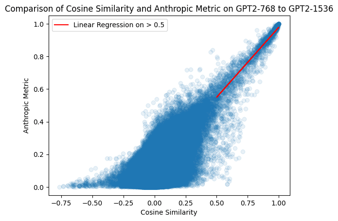
To evaluate whether features are similar or dissimilar between SAEs trained on the same layer, we use the cosine similarity of the decoder directions for those features. Nanda [AF · GW] proposes using the decoder directions to identify features rather than the encoder weights, as encoder weights are optimized to minimize interference with other features as well as just detecting features, whereas decoder weights define the downstream impact of feature activations. The cosine similarity between two features is calculated as
Towards Monosemanticity uses a masked activation cosine similarity metric, essentially looking at how much the features co-occurred, i.e. activated on the same data points to identify similar features. However, we empirically find a high correlation between this metric and the decoder cosine similarity metric for similar features, and decoder cosine similarity is considerably computationally cheaper.
To find the features in GPT2-768 that are most similar to each feature in GPT2-1536, we iterate over each feature in GPT2-1536, take the cosine sim with each feature in GPT-768 and take the max cosine sim. (Note that this metric is not symmetric, if we do it for GPT-768 on GPT-1536 we get 768 numbers not 1536 numbers)
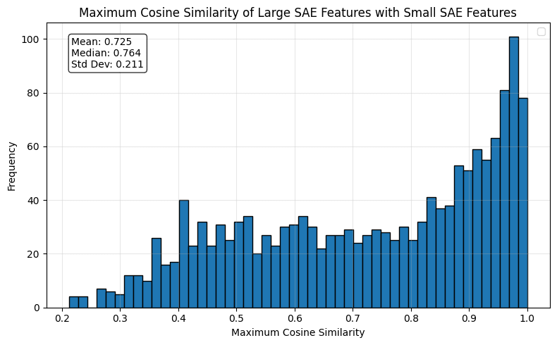
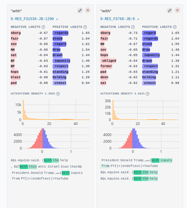
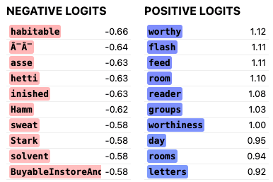
On the right-hand-side there is a cluster of GPT2-1536 features with high cosine similarity to at least one of the GPT2-768 features. For example, GPT2-1536:1290 (left) and GPT2-768:0 (right) have a cosine similarity of 0.99, and both activate strongly on the token “with” and boost similar logits, with some overlap in their max activating dataset.
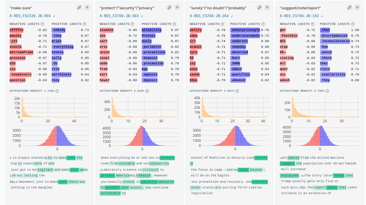
However, the GPT2-1536 feature GPT2-1536:903 that activates on “make sure” has no counterpart in the 768 feature SAE. The three closest features in the 768-feature SAE are:
- “suggest/note/report” (decoder cosine sim 0.352) GPT2-768:192
- “surely”/”no doubt”/”probably” (decoder cosine sim 0.301) - GPT2-768:264
- “protect”/”security”/”privacy” (decoder cosine sim 0.299)- GPT2-768:303
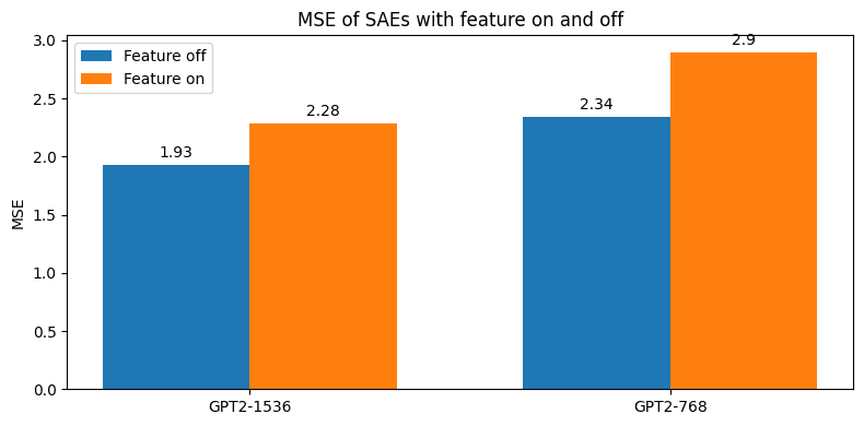
If we compare the reconstruction of the two SAEs on dataset examples where GPT2-1536:903 is active vs inactive, we find the difference in MSE is significantly larger in the small SAE, confirming the novel information added by this feature is not present in GPT2-768.
| Feature inactive | Feature active | Difference | |
| GPT2-1536 | 2.225 | 2.518 | 0.293 |
| GPT2-768 | 2.703 | 3.292 | 0.589 |
Averaging this metric across all 657 features in GPT-1536 that have low maximum cosine similarity (<=0.7) with all features in GPT-768 we see a similar pattern.
Can we add features from one SAE to another?
We evaluate whether it is possible to add features from one SAE into another SAE without decreasing, and ideally improving, reconstruction performance. Given two base SAEs:
and
We can construct a hybrid SAE by adding a feature from one to the other. For example we can add feature 3 from to :
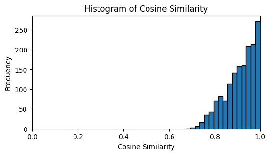
To test if the novel features from larger SAEs can improve smaller SAEs, we add each feature from GPT2-1536 into GPT2-768 one at a time and measure the change in MSE. We find a clear relationship between a feature's maximum cosine similarity to GPT2-768 and its impact on MSE. Features with a smaller maximum cosine similarity almost universally improve performance, while adding more similar features tend to hurt performance.
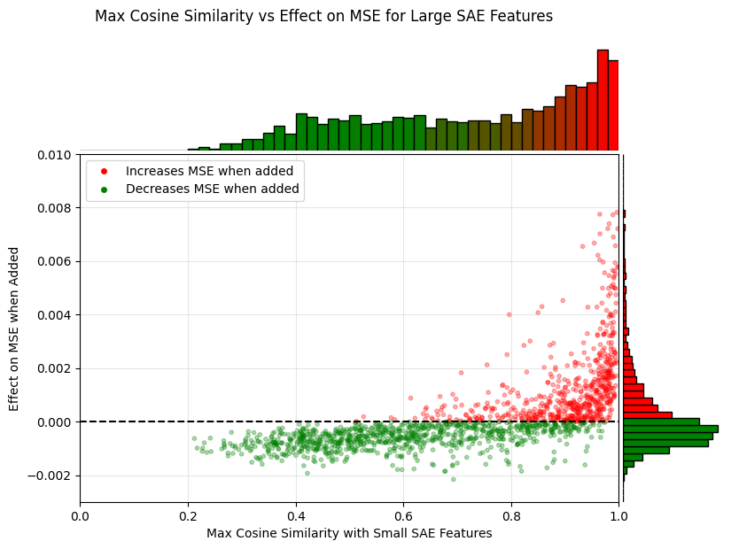
Based on the results we divide the features of a larger SAE in two groups, using a maximum cosine similarity threshold of 0.7. This threshold is chosen somewhat arbitrarily, but seems to be around the point where the majority of features change from decreasing MSE to increasing MSE. Furthermore, it is close to , which is the cosine similarity threshold where the vectors are more aligned than orthogonal.
Based on this threshold we divide the features in two categories:
- Novel features:
- Max cosine similarity <= 0.7 with the smaller SAE
- Reconstruct information that was not reconstructed in the smaller SAE
- Mostly reduce the MSE component of the loss
- Can be added to the smaller SAE and decreases MSE
- Reconstruction features:
- Max cosine similarity > 0.7 with the smaller SAE
- Reconstruct similar features as the smaller SAE
- Mostly reduce the sparsity component of the loss
- Cannot be added to the smaller SAE without increasing MSE
| Novel features | Reconstruction features | |
| ∂ MSE < 0 | 628 | 281 |
| ∂ MSE > 0 | 29 | 598 |
The reason that many of the reconstruction features with high cosine similarity (> 0.7) increase MSE is that their information is already well-represented in the smaller SAE. Adding them causes the model to overpredict these features, impairing reconstruction performance. In contrast, novel features with lower cosine similarity (<= 0.7) mostly provide new information that was not captured by the smaller SAE, leading to improved reconstruction when added.
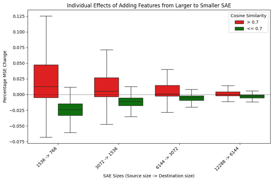
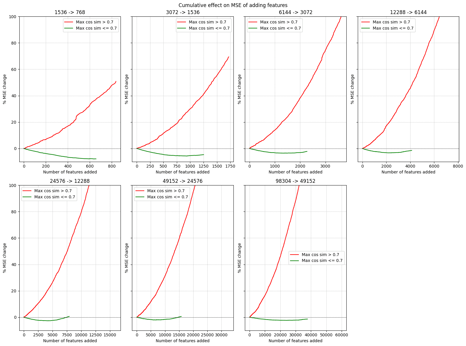
The figures above further supports this categorization into two groups based on the maximum cosine similarity. We see a clear difference in both the individual effect of adding in a reconstruction feature vs a novel feature as well as a difference in the cumulative effect of adding in all novel or reconstruction features. We can decrease the MSE of GPT2-768 by almost 10% by just adding in 657 features from GPT-1536 to GPT-768.
Can we swap features between SAEs?
In the previous section, we saw that adding novel features from larger SAEs to smaller SAEs can improve the performance of the smaller SAEs. However, we can't simply add in all features from the larger SAE, as some of them represent information that is already captured by the smaller SAE (reconstruction features). Instead, we can swap these similar features between the SAEs.
To identify which features can be swapped with which other features, we apply the same threshold to the decoder cosine similarity metric as before. If the cosine similarity between a large SAE feature and a small SAE feature is greater than 0.7, we consider the large SAE feature to be a child of the small SAE feature. This allows us to construct a graph of relationships between features in the small and large SAEs, where connected subgraphs represent potential swaps. These structures are very similar to the feature splitting phenomenon as shown in Towards Monosemanticity.
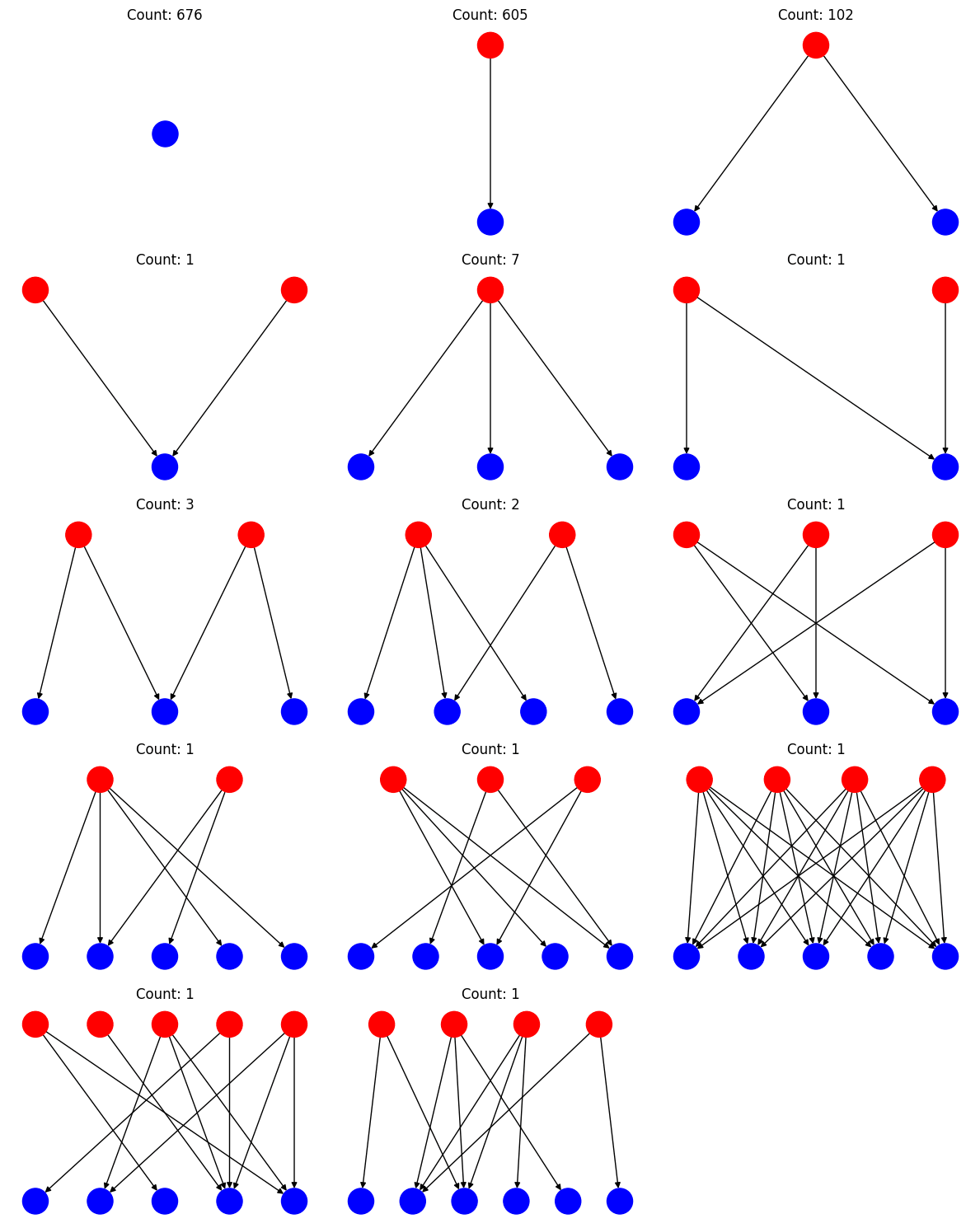
Based on these proposed swaps, we can replace the parents in the small SAE with their children (reconstruction features) in the larger SAE to get a more sparse representation without impacting the MSE too much. Most of the swaps result individually in an increase in MSE, but also in a decrease of L0.
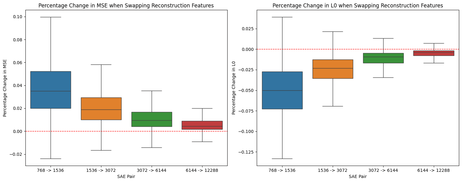
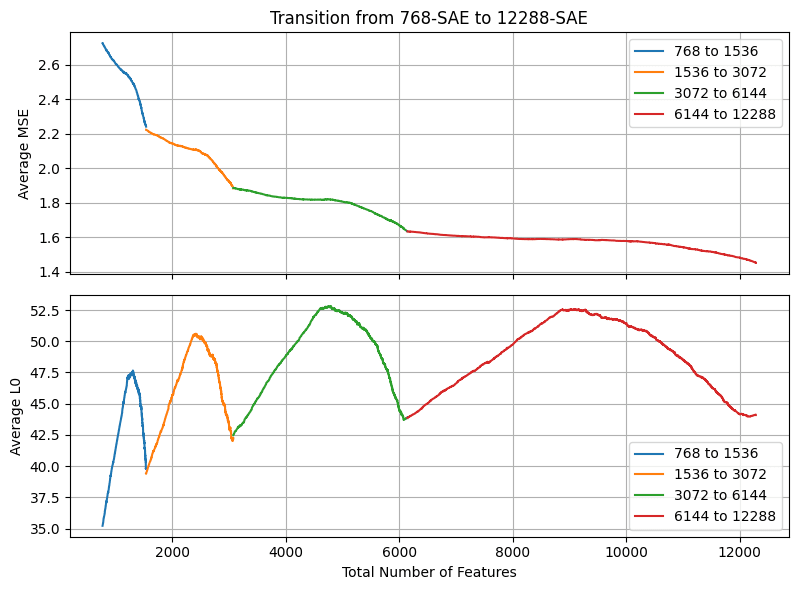
Now if we combine these two methods and first add in all the novel features and then swap the reconstruction features in order of cosine similarity, we can smoothly interpolate between two SAE sizes. In this way, we have many possibilities to select a model with different trade-offs between the number of features, reconstruction performance, and L0.
Frankenstein’s SAE
In the previous section we saw that adding in parentless SAE features from large SAEs improves the performance of smaller SAEs. We now investigate whether this insight can be used to create smaller SAEs with a lower loss than the original SAEs. The idea here is to iteratively take the features from SAEs that add new information and to create a new SAE by stitching all these features together: Frankenstein’s SAE.
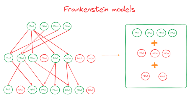
We construct Frankenstein’s SAEs in the following way:
- Start out with a base model (in our case the 768-feature SAE)
- For all other SAEs up to a certain size:
- Select all features that have a cosine similarity of < 0.7 to all features in the current Frankenstein model
- Add these features to the current Frankenstein model
- Repeat for the next largest SAE
- Retrain the decoder weights for 100M tokens[1]
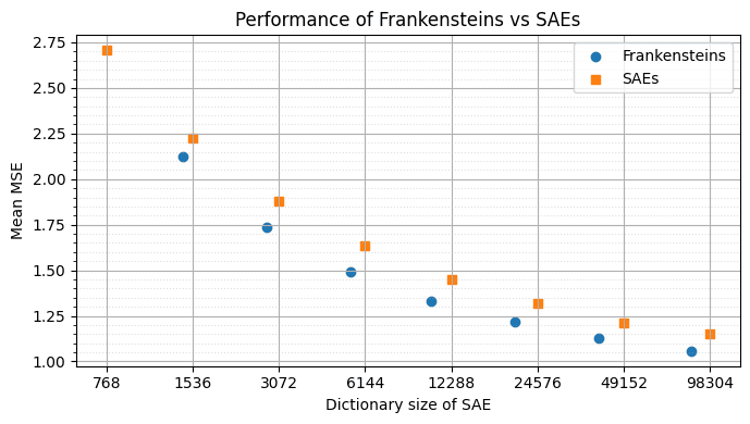
This allows us to construct sparse autoencoders with lower MSE reconstruction loss than the original SAEs of the same size. Frankenstein's SAE with 40214 features already has a better reconstruction performance than the original SAE with 98304 features! This is partly explained by the fact that the Frankenstein SAEs have a much higher L0, as we keep adding in all the novel features without swapping in the sparsifying reconstruction features. For example, the Frankenstein SAE with 1425 features has an L0 of 53.1 (vs an L0 of 35.0 for the normal SAE of size 1536) and the Frankenstein with 10485 features has an L0 109.7 (vs 44.1 for the SAE with dictionary size 12288). If we would simply train an autoencoder with a lower sparsity penalty, this will also result in a model with higher L0 and lower MSE. However, we argue that the features in the Frankenstein model may be more interpretable than those learned by a regular sparse autoencoder with high L0. Firstly, the encoder directions are unchanged from those of the features in the original SAEs, and thus activate exactly on the same examples as the low-L0 SAEs. Secondly, the fine-tuned decoder directions have high cosine similarity to features in the base SAEs.
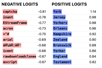
Even the features with low cosine similarity have clear and similar interpretations. For example, feature 867 (left) in the frankenstein SAE has 0.73 cosine similarity with its GPT2-1536:183 origin (right), however it boosts largely the same logits.
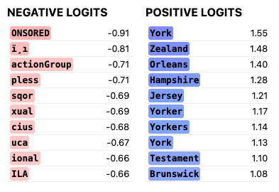
Similarly, frankenstein features 1128 (left) and GPT-1536:662 (right), with a cosine similarity of 0.74.

Although we have to train a number of SAEs to achieve the same performance as a larger SAE, the total number of features trained is the same. For example, constructing our SAE with 40124 features required training SAEs with
features, slightly fewer than in the largest SAE (98304 features).
Discussion and Limitations
In this brief investigation, we found that when you scale up SAEs, they effectively learn two groups of features. One group consists of entirely novel features, which we can add into smaller SAEs which boosts their performance. The second group is of features that are reconstructions of features present in the smaller SAE, and that we can swap into the smaller SAE to decrease the L0.
We used these insights to construct "Frankenstein" SAEs, which stitch together novel features from multiple pre-trained SAEs of different sizes. By iteratively adding in novel features and retraining the decoder, we were able to construct SAEs with lower reconstruction loss than original SAEs with the same number of features (at the cost of a higher L0).
There are several limitations to this work:
- The choice of metrics (decoder cosine similarity) and thresholds (0.7) used to categorize features as novel vs reconstruction features was somewhat arbitrary. More principled and robust methods for identifying feature similarity across SAEs would be valuable. Other measures might provide a cleaner split between “novel features” and “reconstruction features”.
- It's unclear how well these findings will generalize to SAEs trained on different model architectures, layers, and training setups. We’ve obtained similar results with the two SAEs trained on Pythia-410M-deduped, but have not tested these techniques on SAEs trained on MLP or attention layers or much larger models.
- It’s not clear how to interpret the results from the Frankenstein models. They perform much better, but also have much higher L0. As there are currently no good metrics for SAE quality, we’re unsure whether low L0 is an aim in itself (in which case the Frankenstein models are likely not very impressive) or just a proxy for interpretability (in which case the Frankenstein models are interesting as their features are as interpretable as the original SAE features).
- The iterative approach based on cosine similarity used to construct Frankenstein SAEs likely produces suboptimal feature sets. More sophisticated methods that consider the marginal effect of each new feature in the context of those already added could yield even better performing SAEs.
- We haven’t looked at how features of different SAE sizes or our Frankenstein SAEs perform on specific tasks, such as IOI or sentiment classification.
Overall, we believe this work provides valuable insights into what happens when you scale up SAEs and introduces a simple approach to stitch features from one SAE to another.
- ^
Without retraining the decoder weights Frankenstein’s SAEs performance starts to degrade when adding in novel features from too many different sizes of SAEs. As the novel features still share some common directions (up to cosine similarity 0.7), adding in too many of these features still leads to the over-prediction of some feature directions.
12 comments
Comments sorted by top scores.
comment by leogao · 2024-07-13T21:02:07.698Z · LW(p) · GW(p)
Cool work - figuring out how much of scaling up autoencoders is discovering new features vs splitting existing ones feels quite important. Especially since for any one scale of autoencoder there are simultaneously features which are split too finely and features which are too rare to yet be discovered, it seems quite plausible that the most useful autoencoders will be ones with features stitched together from multiple scales.
Some minor nitpicks: I would recommend always thinking of MSE/L0 in terms of the frontier between the two, rather than either alone; in my experiments I found it very easy to misjudge at a glance whether a run with better MSE but worse L0 was better or worse than the frontier.
Replies from: Stuckwork↑ comment by Bart Bussmann (Stuckwork) · 2024-07-13T22:01:56.017Z · LW(p) · GW(p)
Thanks!
Yeah, I think that's fair and don't necessarily think that stitching multiple SAEs is a great way to move the pareto frontier of MSE/L0 (although some tentative experiments showed they might serve as a good initialization if retrained completely).
However, I don't think that low L0 should be a goal in itself when training SAEs as L0 mainly serves as a proxy for the interpretability of the features, by lack of good other feature quality metrics. As stitching features doesn't change the interpretability of the features, I'm not sure how useful/important the L0 metric still is in this context.
comment by RogerDearnaley (roger-d-1) · 2024-07-17T03:09:10.242Z · LW(p) · GW(p)
What I would be interested to understand about feature splitting is whether the fine-grained features are alternatives, describing an ontology, or are defining a subspace (corners of a simplex, like R, G, and B defining color space). Suppose a feature X in a small VAE is split into three features X1, X2, and X3 in a larger VAE for the same model. If occurrences of X1, X2, and X3 are correlated, so activations containing any of them commonly have some mix of them, then they span a 2d subspace (in this case the simplex is a triangle). If, on the other hand, X1, X2 and X3 co-occur in an activations only rarely (just as two randomly-selected features rarely co-occur), then they describe three similar-but-distinct variations on a concept, and X is the result of coarse-graining these together as a singly concept at a higher level in an ontology tree (so by comparing VAEs of different sizes we can generate a natural ontology).
This seems like it would be a fairly simple, objective experiment to carry out. (Maybe someone already has, and can tell me the result!) It is of course quite possible that some split features describe subspaces, and other ontologies, or indeed something between the two where the features co-occur rarely but less rarely than two random features. Or X1 could be distinct but X2 and X3 might blend to span a 1-d subspace. Nevertheless, understanding the relative frequency of these different behaviors would be enlightening.
It would be interesting to validate this using a case like the days of the week, where we believe we already understand the answer: they are 7 alternatives that are laid out in a heptagon in a 2-dimensional subspace that enables doing modular addition/subtraction modulo 7. So if we have a VAE small enough that it represented all day-of-the week names by a single feature, if we increase the VAE size somewhat we'd expect to see this to split into three features spanning a 2-d subspace, then if we increased it more we'd expect to see it resolve into 7 mutually-exclusive alternatives, and hopefully then stay at 7 in larger VAEs (at least until other concepts started to get mixed in, if that ever happened).
Replies from: Stuckwork↑ comment by Bart Bussmann (Stuckwork) · 2024-07-18T03:25:38.621Z · LW(p) · GW(p)
Yes! This is indeed a direction that we're also very interested in and currently working on.
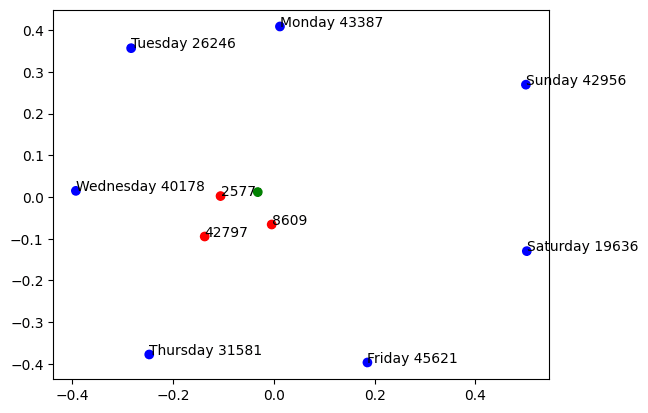
As a sneak preview regarding the days of the week, we indeed find that one weekday feature in the 768-feature SAE, splits into the individual days of the week in the 49152-feature sae, for example Monday, Tuesday..
The weekday feature seems close to mean of the individual day features.
↑ comment by RogerDearnaley (roger-d-1) · 2024-07-22T23:48:48.659Z · LW(p) · GW(p)
Cool! That makes a lot of sense. So does it in fact split into three before it splits into 7, as I predicted based on dimensionality? I see a green dot, three red dots, and seven blue ones… On the other hand, the triangle formed by the three red dots is a lot smaller than the heptagram, which I wasn't expecting…
I notice it's also an oddly shaped heptagram.
↑ comment by Patrick Leask (patrickleask) · 2024-07-24T00:07:17.360Z · LW(p) · GW(p)
Not quite - the green dot is the weekday feature from the 768 SAE, the blue dots are features from the ~50k SAE that activate on strictly one day of the week, and the red dots are multi-day features.
comment by samshap · 2024-07-14T23:53:13.903Z · LW(p) · GW(p)
:Here's my longer reply.
I'm extremely excited by the work in SAEs and their potential for interpretability, however I think there is a subtle misalignment in the SAE architecture and loss function, and the actual desired objective function.
The SAE loss function is:
, where is the -Norm.
or
I would argue that, however, what you are actually trying to solve is the sparse coding problem:
where, importantly, the inner optimization is solved separately (including at runtime).
Since is an overcomplete basis, finding that minimizes the inner loop (also known as basis pursuit denoising[1] ) is a notoriously challenging problem, one which a single-layer encoder is underpowered to compute. The SAE's encoder thus introduces a significant error , which means that you are actual loss function is:
The magnitude of the errors would have to be determined empirically, but I suspect that it is enough to be a significant source of error..
There are a few things you could do reduce the error:
- Ensuring that obeys the restricted isometry property[2] (i.e. a cap on the cosine similarity of decoder weights), or barring that, adding a term to your loss function that at least minimizes the cosine similarities.
- Adding extra layers to your encoder, so it's better at solving for .
- Empirical studies to see how large the feature error is / how much reconstruction error it is adding.
- ^
https://epubs.siam.org/doi/abs/10.1137/S003614450037906X?casa_token=E-R-1D55k-wAAAAA:DB1SABlJH5NgtxkRlxpDc_4IOuJ4SjBm5-dLTeZd7J-pnTAA4VQQ2FJ6TfkRpZ3c93MNrpHddcI
- ^
http://www.numdam.org/item/10.1016/j.crma.2008.03.014.pdf
↑ comment by Neel Nanda (neel-nanda-1) · 2024-07-15T20:44:58.778Z · LW(p) · GW(p)
Interesting! You might be interested in a post from my team [? · GW] on inference-time optimization
It's not clear to me what the right call here is though, because you want f to be something the model could extract. The encoder being so simple is in some ways a feature, not a bug - I wouldn't want it to be eg a deep model, because the LLM can't easily extract that!
Replies from: samshap↑ comment by samshap · 2024-07-16T21:49:00.494Z · LW(p) · GW(p)
Thanks for sharing that study. It looks like your team is already well-versed in this subject!
You wouldn't want something that's too hard to extract, but I think restricting yourself to a single encoder layer is too conservative - LLMs don't have to be able to fully extract the information from a layer in a single step.
I'd be curious to see how much closer a two-layer encoder would get to the ITO results.
comment by Dan Braun (dan-braun-1) · 2024-07-15T12:21:16.935Z · LW(p) · GW(p)
Excited by this direction! I think it would be nice to run your analysis on SAEs that are the same size but have different seeds (for dataset and parameter initialisation). It would be interesting to compare how the proportion and raw number of "new info features" and "similar info features" differ between same size SAEs and larger SAEs.
comment by samshap · 2024-07-13T22:12:16.829Z · LW(p) · GW(p)
This is great work. My recommendation: add a term in your loss function that penalizes features with high cosine similarity.
I think there is a strong theoretical underpinning for the results you are seeing.
I might try to reach out directly - some of my own academic work is directly relevant here.
Replies from: Stuckwork↑ comment by Bart Bussmann (Stuckwork) · 2024-07-13T22:40:16.518Z · LW(p) · GW(p)
Interesting! I actually did a small experiment [LW(p) · GW(p)] with this a while ago, but never really followed up on it.
I would be interested to hear about your theoretical work in this space, so sent you a DM :)