the scaling “inconsistency”: openAI’s new insight

post by nostalgebraist · 2020-11-07T07:40:06.548Z · LW · GW · 14 comments

Contents

  1. L(C) and L(D)
  2. C sets E, and E bounds D
    Budget tradeoffs
    From step count to update count
    From update count to data count
  3. The inconsistency
    L(D): information
    L(C): budgeting
    N goes up fast, S goes up slowly…
    … and you claim to achieve the impossible
  4. The resolution
    Bigger models extract a resource faster
    The resource is finite
    Converging in the very first step
    Getting a bigger quarry
    Where we are now
  Implications
None
14 comments

I’ve now read the new OpenAI scaling laws paper.  Also, yesterday I attended a fun and informative lecture/discussion with one of the authors.

While the topic is on my mind, I should probably jot down some of my thoughts.

This post is mostly about what the new paper says about the “inconsistency” brought up in their previous paper.

The new paper has a new argument on this topic, which is intuitive and appealing, and suggests that the current scaling trend will indeed “switch over” soon to a new one where dataset size, not model size, is the active constraint on performance.  Most of this post is an attempt to explain and better understand this argument.

——

The new paper is mainly about extending the scaling laws from their earlier paper to new modalities.

In that paper, they found scaling laws for transformers trained autoregressively on text data.  The new paper finds the same patterns in the scaling behavior of transformers trained autoregressively on images, math problems, etc.

So the laws aren’t telling us something about the distribution of text data, but about something more fundamental.  That’s cool.

They also have a new, very intuitive hypothesis for what’s going on with the “scaling inconsistency” they described in the previous paper – the one I made a big deal about at the time.  So that’s the part I’m most excited to discuss.

I’m going to give a long explanation of it, way longer than the relevant part of their paper.  Some of this is original to me, all errors are mine, all the usual caveats.

——

1. L(C) and L(D)

To recap: the “inconsistency” is between two scaling laws:

• The law for the best you can do, given a fixed compute budget.
  
  This is L(C), sometimes called L(C_min).  L is the loss (lower = better), C is your compute budget.
  
  
• The law for the best you can do, given a fixed dataset size.
  
  This is L(D), where D is the number of examples (say, tokens) in the dataset.
  

Once you reach a certain level of compute, these two laws contradict each other.

I’ll take some time to unpack that here, as it’s not immediately obvious the two can even be compared to one another – one is a function of compute, the other of data.

2. C sets E, and E bounds D

Budget tradeoffs

Given a compute budget C, you can derive the optimal way to spend it on different things.  Roughly, you are trading off between two ways to spend compute:

• Use C to buy “N”: Training a bigger model – “N” here is model size
  
  
• Use C to buy “S”: Training for more steps “S” (gradient updates)

The relationship between S (steps) and D (dataset size) is a little subtle, for several reasons.

From step count to update count

For one thing, each single “step” is an update on the information from more than one data point.  Specifically, a step updates on “B” different points – B is the batch size.

So the total number of data points processed during training is B times S.  The papers sometimes call this quantity “E” (number of examples), so I’ll call it that too.

From update count to data count

Now, when you train an ML model, you usually update on each data point more than once.  Typically, you’ll do one pass over the full dataset (updating on each point as you go along), then you’ll go back and do a second full pass, and then a third, etc.  These passes are called “epochs.”

If you’re doing things this way, then for every point in the data, you get (number of epochs) updates out of it.  So

E = (number of epochs) * D.  

Some training routines don’t visit every point the exact same number of times – there’s nothing forcing you to do that.  Still, for any training procedure, we can look at the quantity E / D.

This would be the number of epochs, if you’re doing epochs.  For a generic training routine, you can can think of E / D as the “effective number of epochs”: the average number of times we visit each point, which may not be an integer.

Generally, E ≠ D, but we always have E≥D.  You can’t do fewer than one epoch; you can’t visit the average point less than once.

This is just a matter of definitions – it’s what “dataset size” means.  If you say you’re training on a million examples, but you only update on 100 individual examples, then you simply aren’t “training on a million examples.”

3. The inconsistency

L(D): information

OpenAI derives a scaling law called L(D).  This law is the best you could possibly do – even with arbitrarily large compute/models – if you are only allowed to train on D data points.

No matter how good your model is, there is only so much it can learn from a finite sample.  L(D) quantifies this intuitive fact (if the model is an autoregressive transformer).

L(C): budgeting

OpenAI also derives another a scaling law called L(C).  This is the best you can do with compute C, if you spend it optimally.

What does optimal spending look like?  Remember, you can spend a unit of compute on 

• a bigger model (N), or 
• training the same model for longer (S)

(Sidenote: you can also spend on bigger batches B.  But – to simplify a long, complicated story – it turns out that there are really just 2 independent knobs to tune among the 3 variables (B, N, S), and OpenAI frames the problem as tuning (N, S) with B already “factored out.”)

In the compute regime we are currently in, making the model bigger is way more effective than taking more steps.

This was one of the punchlines of the first of these two papers: the usual strategy, where you pick a model and then train it until it’s as good as it can get, is actually a suboptimal use of compute.  If you have enough compute to train the model for that long (“until convergence”), then you have enough compute to train a bigger model for fewer steps, and that is a better choice.

This is kind of counterintuitive!  It means that you should stop training your model before it stops getting better.  (“Early stopping” means training your model until it stops getting better, so this is sort of “extra-early stopping.”)  It’s not that those extra steps wouldn’t help – it’s that, if you are capable of doing them, then you are also capable of doing something else that is better.

Here’s something cool: in Appendix B.2 of the first paper, they actually quantify exactly how much performance you should sacrifice this way.  Turns out you should always stop at a test loss about 10% higher than what your model could asymptotically achieve.  (This will be relevant later, BTW.)

Anyway, OpenAI derives the optimal way to manage the tradeoff between N and S.  Using this optimal plan, you can derive L(C) – the test loss you can achieve with compute C, if you allocate it optimally.

N goes up fast, S goes up slowly…

The optimal plan spends most incremental units of compute on bigger models (N).  It spends very little on more steps (S).

The amount it spends on batch size (B) is somewhere in between, but still small enough that the product E = B*S grows slowly.

But remember, we know a relationship between E and “D,” dataset size.  E can’t possibly be smaller than D.

So when your optimal plan chooses its B and its S, it has expressed an opinion about how big its training dataset is.

The dataset could be smaller than B*S, if we’re doing many (effective) epochs over it.  But it can’t be any bigger than B*S: you can’t do fewer than one epoch.

… and you claim to achieve the impossible

L(C), the loss with optimally allocated C, goes down very quickly as C grows.  Meanwhile, the dataset you’re training with that compute stays almost the same size.

But there’s a minimum loss, L(D), you can possibly achieve with D data points.

The compute-optimal plan claims “by training on at most B*S data points, with model size N, I can achieve loss L(C).”

The information bound says “if you train on at most B*S data points, your loss can’t get any lower than the function L(D), evaluated at D = B*S.”

Eventually, with enough compute, the L(C) of the compute-optimal plan is lower than the L(D) of the dataset used by that same plan.

That is, even if the compute-optimal model is only training for a single epoch, it is claiming to extract more value that epoch than any model could ever achieve, given any number of epochs.

That’s the inconsistency.

4. The resolution

In the new paper, there’s an intuitive hypothesis for what’s going on here.  I don’t think it really needs the multimodal results to motivate it – it’s a hypothesis that could have been conceived earlier on, but just wasn’t.

Bigger models extract a resource faster

The idea is this.  As models get bigger, they get more update-efficient: each time they update on a data point, they get more out of it.  You have to train them for fewer (effective) epochs, all else being equal.

This fact drives the choice to scale up the model, rather than scaling up steps.  Scaling up the model makes your steps more valuable, so when you choose to scale the model rather than the steps, it’s almost like you’re getting more steps anyway.  (More “step-power,” or something.)

The resource is finite

Each data point has some information which a model can learn from it.  Finite models, trained for a finite amount of time, will miss out on some of this information.

You can think about the total extractable information in a data point by thinking about what an infinitely big model, trained forever, would eventually learn from that point.  It would extract all the information – which is more than a lesser model could extract, but still finite.  (A single data point doesn’t contain all the information in the universe.)

This is literally the definition of L(D): what an infinitely big model, trained forever, could learn from D separate data points.  L(D) quantifies the total extractable information of those points.

(More precisely, the total extractable information is the gap between L(D) and the loss achieved by a maximally ignorant model, or something like that.)

Converging in the very first step

As models get bigger, they extract more information per update.  That is, each time they see a data point, they extract a larger fraction of its total extractable information.

Eventually, your models are getting most of that information the very first time they see the data point.  The “most” in that sentence gets closer and closer to 100%, asymptotically.

How does this relate to optimal compute allocation?

The logic of the “optimal compute plan” is as follows:

Your model is an imperfect resource extractor: it only gets some of the resources locked up in a data point from the first update.  So you could extract more by running for more steps … 

…  but if you have the compute for that, you can also spend it by making your steps more efficient.  And, in the current compute regime, that’s the smarter choice.

It’s smarter by a specific, uniform proportion.  Remember, you should stop training when your loss is 10% higher than the converged loss of the same model.  If the converged loss is L, you should stop at 1.1*L.

Can you always do that?  If your model is efficient enough, you can’t!  As the first epoch gets closer to 100% efficient, the loss after the first epoch gets arbitrarily close to the converged loss.  Your loss goes under 1.1*L by the end of the first epoch.

At this point, the story justifying the L(C) law breaks down.

The L(C) law goes as fast is it does because upgrading the efficiency of your extractor is cheaper – in terms of compute spent per unit of resource extracted – than actually running the extractor.

This works as long as your extractor is inefficient.  But you can’t push efficiency above 100%.  Eventually, the only way to extract more is to actually run the damn thing.

Getting a bigger quarry

When you’re extracting a resource, there’s a difference between “improve the extractor” and “get a bigger quarry.”

If your quarry has 100 resource units in it, the strategy of “improving the extractor” can never get you more than 100 units.  It can get them to you faster, but if you want more than 100 units, you have to get a bigger quarry.

“N” sets the efficiency of the extractor.  “S” sets … well, it doesn’t exactly set the size of the quarry (that’s D).  There is an ambiguity in the S: it could mean running for more epochs on the same data, or it could mean getting more data.

But S does, at least, set an upper bound on the size of the quarry, D.  (Via D≤E and E = B*S, with B set optimally as always.)

With high enough compute (and thus model size), you’ve pushed the “extractor upgrades are cheap” lifehack as far as it can go.  With this efficient extractor, taking S steps (thus making E = B*S updates) sucks up most of the information theoretically extractable from E individual data points.

The learning curve L(E) of your model, as it makes its first pass over the dataset, starts to merge with L(D), the theoretical optimum achievable with that same dataset.  You trace out L(D) as you train, and the relevant constraint on your performance is the maximum data size D you can obtain and train on.

Where we are now

In the compute regime that spans GPT-2 and the smaller variants of GPT-3, extraction is far less than maximally efficient.  The L(C) strategy applies, and the smart move is to spend compute mostly on model size.  So you make GPT-2, and then GPT-3.

Once we get to the full GPT-3, though, the extractor is efficient enough that the justification for L(C) has broken down, and the learning curve L(E) over the first epoch looks like L(D).

Here is that as a picture, from the new paper:

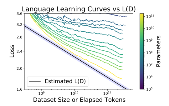
The yellowest, lowest learning curve is the full GPT-3.  (The biggest GPT-2 is one of the green-ish lines.)  The black line is L(D), maximally efficient extraction.

You can see the whole story in this picture.  If you’re in one of the smaller-model learning curves, running for more steps on more data will get you nowhere near to the total extractable info in that data.  It’s a better use of your compute to move downwards, toward the learning curve of a bigger model.  That’s the L(C) story.

If the L(C) story went on forever, the curves would get steeper and steeper.  Somewhere a little beyond GPT-3, they would be steeper than L(D).  They would cross L(D), and we’d be learning more than L(D) says is theoretically present in the data.

According to the story above, that won’t happen.  We’ll just converge ever closer to L(D).  To push loss further downward, we need more data.

Implications

Since people are talking about bitter lessons a lot these days, I should make the following explicit: none of this means “the scaling hypothesis is false,” or anything like that.

It just suggests the relevant variable to scale with compute will switch: we’ll spent less of our marginal compute on bigger models, and more of it on bigger data.

That said, if the above is true (which it may not be), it does suggest that scaling transformers on text alone will not continue productively much past GPT-3.

The GPT-3 paper says its choices were guided by the “grow N, not S” heuristic behind the L(C) curve:

Based on the analysis in Scaling Laws For Neural Language Models [KMH+20] we train much larger models on many fewer tokens than is typical.

(“KMH+20″ is the first of the two scaling papers discussed here.)  Even following this heuristic, they still picked a huge dataset, by human standards for text datasets.

In the above terms, their “E” was 300 billion tokens and their “D” was ~238 tokens, since they updated multiple times on some tokens (cf. Table 2.2 in the GPT-3 paper).  The whole of Common Crawl is 410 billion tokens, and Common Crawl might as well be “all the text in the universe” from the vantage point of you and me.

So, there’s room to scale D up somewhat further than they did with GPT-3, but not many orders of magnitude more.  To me, this suggests that an intuitively “smarter” GPT-4 would need to get its smartness from being multimodal, as we really can’t go much further with just text.

14 comments

Comments sorted by top scores.