Infra-Bayesian haggling

post by hannagabor (hanna-gabor) · 2024-05-20T12:23:30.165Z · LW · GW · 0 comments

Contents

  Preface
  Introduction
  Preliminaries
    Repeated games
    Running example: Prisoner's dilemma
    Other notation
  Proposed algorithm
  How to describe hypotheses?
    Regular decision processes
    Resettable infra-RDPs
    Which hypotheses are in the hypothesis space of the agents?
  Learning-theoretic guarantee
  Where does following this algorithm lead the agents?
    Generalized stag hunt - unique Pareto-optimal outcome
        Reasoning behind the Conjecture:
    Prisoner's dilemma
    Schelling Pub (Battle of the sexes)
    Schelling points
    Multiplayer games
      When can a coalition be formed?
      Stable cycles for multiplayer games
  Conclusion
  Future directions
  Appendix
None
No comments

Preface

I wrote this post during my scholarship at MATS. My goal is to describe a research direction of the learning theoretic agenda [LW · GW] (LTA). Namely, a natural infra-Bayesian learning algorithm proposal that arguably leads to Pareto-optimal solutions in repeated games. The idea originates from Vanessa, I'm expanding a draft of her into a more accessible description.

The expected audience are people who are interested in ongoing work on LTA. It is especially suitable for people who are looking for a research direction to pursue in this area.

Introduction

There has been much work on the theory of agents who cooperate in the Prisoner's dilemma and other situations. Some call this behavior superrationality [? · GW]. For example, functional decision theory (FDT) is a decision theory that prescribes such behavior. The strongest results so far are those coming from "modal combat", e.g. Critch. However, these results are of very limited scope: among other issues, they describe agents crafted for specific games, rather than general reasoners that produce superrational behavior in a "naturalized" manner (i.e. as a special case of the general rules of reasoning.)

At the same time, understanding multi-agent learning theory is another major open problem. Attempts to prove convergence to game-theoretic solution concepts (a much weaker goal than superrationality) in a learning-theoretic setting are impeded by the so-called grain-of-truth problem (originally observed by Kalai and Lehrer, its importance was emphasized by Hutter). An agent can learn to predict the environment via Bayesian learning only if it assigns non-zero prior probability to that environment, i.e. its prior contains a grain of truth. What's the grain-of-truth problem? Suppose Alice's environment contains another agent, Bob. If Alice is a Bayesian agent, she can learn to predict Bob's behavior only if her prior assigns a positive probability to Bob's behavior. (That is, Alice's prior contains a grain of truth.) If Bob has the same complexity level as Alice, then Alice is not able to represent all possible environments. Thus, in general, Alice's prior doesn't contain a grain of truth. A potential solution based on "reflective oracles" was proposed by Leike, Taylor and Fallenstein. However it involves arbitrarily choosing a fixed point out of an enormous space of possibilities, and requires that all agents involved choose the same fixed point. Approaches to multi-agent learning in the mainstream literature (see e.g. Cesa-Bianchi and Lugosi) also suffer from restrictive assumptions and are not naturalized.

Infra-Bayesianism [LW · GW] (IB) was originally motivated by the problem of non-realizability, of which the multi-agent grain-of-truth problem is a special case. Moreover, it converges to FDT-optimal behavior in most Newcombian problems [? · GW]. Therefore, it seems natural to expect IB agents to have strong multi-agent guarantees as well, hopefully even superrationality.

In this article, we will argue that an infra-Bayesian agent playing a repeated game displays a behavior dubbed "infra-Bayesian haggling". For two-player games, this typically (but, strictly speaking, not always) leads to Pareto-efficient outcome. The latter can be a viewed as a form of superrationality. Currently, we only have an informal sketch, and even that in a toy model with no stochastic hypotheses. However, it seems plausible that it can be extended to a fairly general setting. Certainly it allows for asymmetric agents with different priors and doesn't have any strong mutual compatibility condition. The biggest impediment to naturality is the requirement that the learning algorithm is of a particular type (namely, Upper Confidence Bound). However, we believe that it should be possible to replace it by some natural abstract condition.

Preliminaries

Repeated games

As mentioned, we will focus our exploration on infinitely repeated games.

Notation: In a $k$-player game, each player $i$ can choose from a finite set of actions $A_i$. Let $A=\prod _{i=1}^k{A}_i$ be the set of action profiles. Furthermore, each player $i$ has a reward function  $r_i:A\to R$.

Contrary to classical game theory, we look at this setting as a reinforcement learning setup. At time step $n$, player $i$ can choose from action set $A_i$, then receives an observation $a_{-i}^{\left(n\right)}\in \prod _{j\ne i}{A}_j$ consisting of the actions played by other players at time step $n$, and reward $r_i\left(a^{\left(n\right)}\right)$. The goal of agent $i$ is to maximize its utility  $u_i=\sum _{n=0}^{\infty }(1-\gamma ){\gamma }^n{r}_i\left(a^{\left(n\right)}\right)$ for some discount factor $\gamma$.

We will use the words "agent" and "player" interchangeably.

Remark: We suppose the agents know the rules of the game. Specifically, this means player $i$ knows the reward function $r_i$, but doesn't necessarily know $r_j$ for $j\ne i$.

Notation:  Let $A_{-i}$ be the set of possible observations for player $i$ : $A_{-i}=\prod _{j\ne i}{A}_j$.

Running example: Prisoner's dilemma

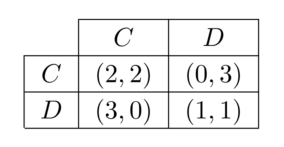
We will use the Prisoner's dilemma [? · GW] to illustrate some of the concepts later in the post. Here, the players can choose between cooperating and defecting and they get the following rewards:

Other notation

We will also use the following notations.

Notation: For set $X$, let $X^{\ast }$ denote the set of finite sequences of elements of $X$: $X^{\ast }=\bigcup _{n=1}^{\infty }{X}^n$.

Notation: For set $X$, let $\Delta$X denote the set of probability distributions on $X$.

Proposed algorithm

Each agent starts with a set of hypotheses $H$ about how the other agents might behave. We will talk about the exact form of these hypotheses in the next section. For now we just assume $H$ is finite and each agent has a prior distribution $\zeta \in \Delta \left(H\right)$ over the hypotheses. Note that we neither require the agents to have the same prior over the hypothesis space nor having the same hypothesis space as the others.

The proposed algorithm is the following:

1. Compute the set of hypotheses that are consistent with our experience so far. Let us denote it with $C$.
2. Find the hypotheses in $C$ that are promising the highest utility, denote this set of hypotheses with $C_{opt}$.
3. Sample an element $h$ from $C_{opt}$ according to the prior $\zeta$ conditioned on $C_{opt}$.
4. Compute the optimal policy $\pi$ if $h$ holds.
5. Follow $\pi$ until $h$ gets falsified. When falsified, go to step 1.

We will discuss how a hypothesis looks like in the next section. Then we will discuss what we mean by "optimal policy"  and "utility" in the section after that.

How to describe hypotheses?

Our first try might be to include all hypotheses of type "Others will play $a_{-i}$", where $a_{-i}\in A_{-i}$. That is way too restrictive. It excludes any dependence on what we have done in previous time steps. It also excludes any probabilistic behavior.

So our second try might be to include hypotheses of type "Others play according to a function $f:A_i^{\ast }\to \Delta A_{-i}$, where $f$ maps histories to distributions on actions of others. This is too fine-grained and intractable.

We need something in between these two extremes. A natural choice would be regular decision processes (RDPs).

Regular decision processes

We will define the hypotheses with the reinforcement learning setting in mind. The "observation" in reinforcement learning is what the agent observes from the environment. In this case, that's the actions the other agents played.

We will slightly abuse notation here. Previously $a$ was an element of  $A=\prod _{i=1}^k{A}_i$ in a $k$-player game. From now on, $a$ will sometimes be an element of the action set of the agent, denoted by $A$. For player $i$,  $A=A_i$.

Definition: A Regular Decision Process (RDP) is a tuple $(S,A,O,s_o,B,T)$, where

• $S$ is a finite set of states
• $A$ is a finite set of actions
• $O$ is a finite set of observations
• $s_0\in S$ is the initial state
• $B:S\times A\to \Delta O$ is the observation kernel that defines a probability distribution over observations for each (state, action) pair
• $T:S\times A\times O\to S$ is the transition function describing the next state after taking action $a$ in state $s$ and observing $o$

Infra-Bayesianism lets us merge some of the RDPs together, which allows us to express beliefs about some aspects of the environment while remaining uncertain about others. (You can read more about infra-Bayesianism here [LW · GW].) The infra-Bayesian version of an RDP is an infra-RDP.

Definition: An Infra-RDP is a tuple $(S,A,O,s_o,B,T)$, where

• $S,A,O,s_o,T$ have the same properties as in an RDP
• $B:S\times A\to \square O$ is the observation kernel, where $\square O$ denotes the convex, closed subsets $\Delta X$. So $B$ defines a closed convex subset of probability distributions over observations for each (state, action) pair.

If you are not familiar with infra-Bayesianism, it is not clear how to interpret this kind of observation kernel. So suppose the environment is in state $s$ and the agent takes action $a$. The hypothesis claims that the next observation is determined by using one of the distributions in $B(s,a)$. This means there exists a probability distribution $\theta :O\to R$, such that $\theta \in B(s,a)$, and the next observation is sampled from $\theta$. Importantly, the hypothesis doesn't say anything about how $\theta$ is chosen from $B(s,a)$: it has Knightian uncertainty about it. $\theta$ could be chosen randomly or could be chosen adversarially by Murphy or using any other method.

In this post, we will focus on a special case of infra-RDPs called sharp infra RDPs. We restrict ourselves to sharp infra-RDPs now to start with an easier special case. However, the hope is that the method described here can be extended to infra-RDPs in future work.

Definition:  A sharp infra-RPD is a tuple $(S,A,O,s_o,B,T)$, where

• $S,A,O,s_o,T$ have the same properties as in an RDP
• $B:S\times A\to 2^O$ is the observation kernel that describes what observations are possible in a particular state given a particular action.

Remark: A sharp infra-RDP is an infra-RDP. The corresponding infra-RDP is defined by the observation kernel $B^{\prime }(s,a)=\{\theta \in \Delta O:supp(\theta )\subseteq B(s,a\left)\right\}$.

Remark: We denote the following special hypothesis with $\top$ (it stands for "top"). There's only one state $s$. Whatever action the agent takes, any observation is possible, that is, $B(s,a)=O$ for any action $a$.
We will assume $\top$ to be in the hypothesis space of each agent. This ensures the agent won't run out of hypotheses: $\top$ will always remain unfalsified. and thus the set of consistent hypotheses $C$ will never be empty.

Remark: For sharp infra-RDPs, there is no ambiguity in deciding whether a hypothesis is falsified or not. For general infra-RDPs we will need to have a statistical notion of whether a hypothesis is falsified or not.

Example: Tit-for-tat is a well-known strategy in the iterated prisoner's dilemma. The strategy is to cooperate in the first round of the game, then do what the agent's opponent did in the previous round. the hypothesis "My opponent follows the tit-for tat strategy " can be represented as a sharp infra-RDP. Actually, this is just a deterministic RDP, there is nothing "infra" in it.

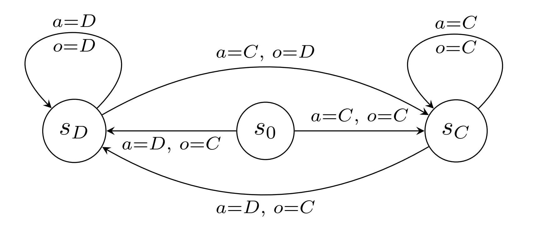
Example: Consider the $\epsilon$-defect strategy in the prisoners dilemma (defect with probability $\epsilon$ and cooperate with probability $1-\epsilon$). This can't be part of the hypothesis space on its own. It is represented as part of $\top$. The closes thing to the $\frac{1}{n}$-defect bot in the agent's hypothesis space is a deterministic bot who cooperates $n-1$ times and then defects once.

Resettable infra-RDPs

In real life, but even in repeated games, there might be irreversible actions, so-called traps. This is a prevalent problem in multi-agent cases, because other agents can have memory. For example, in the prisoners' dilemma, the other player might use the Grim strategy: start with cooperate, but once the other defects, defect forever. In this case, if you defect on the first try, you will never be able to get a reward bigger than 1.

However, for the proposed algorithm to make sense, the agents need to be able to try hypotheses without ruining their chances in any of their other hypotheses. There are weaker conditions that are sufficient, but resettability is enough for our purposes here.

Definition: An infra-RDP $(S,A,O,s_o,B,T)$ is resettable if for all $s\in S$, there exists a policy $\pi :S\to A$, such that if the agent is in $s$ and follows $\pi$, it will eventually reach $s_0.$

Which hypotheses are in the hypothesis space of the agents?

As mentioned previously, we suppose $\top$ is in the hypothesis space. There is an infinite number of sharp infra-RDPs that can potentially be in the agents' hypothesis spaces. We imagine the agents to have some kind of complexity prior and keep all the hypotheses with complexity under a specific threshold. The hope here is that if the prior assigns "enough" probability mass to a special kind of hypotheses, then the agents will end up close to a Pareto-optimal payoff.

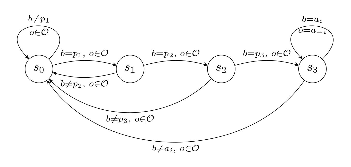
Definition: Suppose there is a unique Pareto-optimal strategy profile $a\in A.$ For $p\in A_i^{\ast }$ of length $n$, we define a simple password hypothesis $h_p$ as the following sharp infra-RDP.

• $S=\{s_0,s_1\dots s_n\}$
• for state $s_k$ and action $b$: $B(s,b)=\{\begin{array}{c}{a}_{-i}\text{if}s=s_n,b=a_i\\ O\text{otherwise}\end{array}$
• for state $s_k$, action $b$ and observation $o$: $T(s_k,b,o)=\{\begin{array}{c}{s}_{k+1}\text{if}k<n,b=p_{k+1}\\ s_n\text{if}k=n,b=a_i\\ s_0\text{otherwise}\end{array}$

That is, if the agent enters the password $p$, the others will play the Pareto-optimal  strategy as long as the agent itself plays the Pareto-optimal action.

Example: For the password $p_1{p}_2{p}_3$ the sharp infra-RDP looks like this:

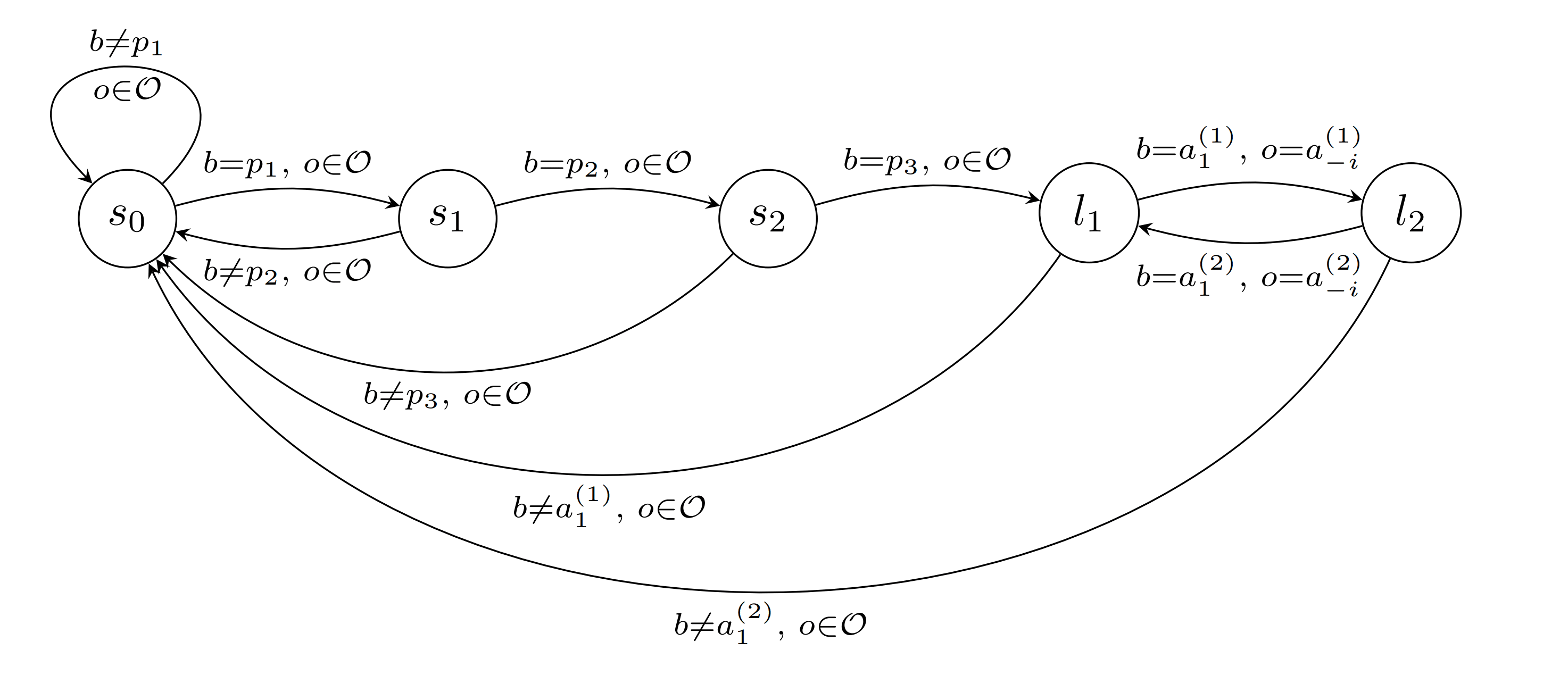
For games where there are multiple Pareto-optimal strategy profiles, a password hypothesis doesn't necessarily end in a unique state. It might end in a loop as well. The idea is that after "entering the password", the world gets into a state where if the agent plays a particular strategy, the other agents are restricted to play a particular strategy as well.

Definition: For a password $p\in \prod ^n{A}_i$ and a sequence $l=a_i^{\left(1\right)},a_{-i}^{\left(1\right)},a_i^{\left(2\right)},a_{-i}^{\left(2\right)}\dots a_i^{\left(m\right)},a_{-i}^{\left(m\right)}\in (A_i\times A_{-i}{)}^{\ast }$, we define the password hypothesis $h_{p,l}$ as the following sharp infra-RDP.

• $S=\{s_0,s_1\dots s_{n-1},l_1,l_2\dots l_m\}$
• The possible set of observations after taking action $b$ in state $s$ are$B(s,b)=\{\begin{array}{c}\left\{a_{-i}^{\left(k\right)}\right\}\text{if}s=l_k,b=a_i^{\left(k\right)}\\ O\text{otherwise}\end{array}$
• The transition for state $s$, action $b$ and observation $o$ is described by $T(s,b,o)=\{\begin{array}{c}{s}_{k+1}\text{if}s=s_k\text{for}k<n-1,b=p_{k+1}\\ l_1\text{if}s=s_{n-1},b=p_n\\ l_{k+1}\text{if}s=l_k,b=a_i^{\left(k\right)}\text{for}k<m-1\\ l_1\text{if}s=l_m,b=a_i^{\left(m\right)}\\ s_0\text{otherwise}\end{array}$

Example For the password $p=p_1{p}_2{p}_3$ and sequence $l=a^{\left(1\right)}{a}^{\left(2\right)}$, the sharp infra-RDP $h_{p,l}$ looks like this:

 

Learning-theoretic guarantee

What can we say about the optimality of this algorithm? In this section, we will show that if the true environment satisfies at least one of the hypotheses in the hypothesis space of the agent, then the agent's payoff converges to at least the optimal payoff of the hypothesis.

What is the optimal payoff of a hypothesis? For a hypothesis $h\in H$, the optimal payoff or value of $h$ is the minimum utility the agent can get if the environment satisfies $h$, and the agent plays the best strategy according to $h$. To define it more formally, we will need to start with what a policy is.

Definition: A stationary policy the agent can play in hypothesis $h$ is an element of ${\Pi }_i^h=\{f:S_h\to A_i\}$. That means a policy is a function that maps states of the sharp infra-RDP to actions.

While following the algorithm, the agent will switch its hypothesis about the world from time to time. The previous definition isn't enough to talk about the agent's behavior including these switches.

Definition: A policy is a function from histories to actions:  $(A_i\times A_{-i}{)}^{\ast }\to A_i$

A copolicy describes the behavior of the other agents. Or in other words, it describes the environment.

Definition: A copolicy in hypothesis $h$ is an element of ${\Pi }_{-i}^h=\{f:(S_h\times A_i\times A_{-i}{)}^{\ast }\times S_h\times A_i\to A_{-i}:f(x,s,a_i)\in B_h(s,a_i)\}$.

Definition: The utility depends on the policy ${\pi }_i$ played, the copolicy ${\pi }_{-i}$ and the discount factor $\gamma$: $u_i({\pi }_i,{\pi }_{-i},\gamma )=\sum _{n=0}^{\infty }(1-\gamma ){\gamma }^n{r}_i\left(a^{\left(n\right)}\right)$

Definition: For discount factor $\gamma$, the value of $h$ is $V_i(h,\gamma )=\underset{{\pi }_i\in {\Pi }_i^h}{max}\underset{{\pi }_{-i}\in {\Pi }_{-i}^h}{min}{u}_i({\pi }_i,{\pi }_{-i},\gamma )$.

Proposition 1: Suppose there is a hypothesis $h$ in the agent's hypothesis space such that the true environment satisfies $h$. Following the proposed algorithm guarantees the expected utility of $V_i(h,\gamma )$ in the $\gamma \to 1$ limit. Let ${\pi }_i$ be the policy defined by the proposed algorithm. Suppose the prior over the hypotheses assigns non-zero weight to $h$. Then $\underset{\gamma \to 1}{lim}\underset{{\pi }_{-i}\in {\Pi }_{-i}^h}{min}{u}_i({\pi }_i,{\pi }_{-i},\gamma )\ge \underset{\gamma \to 1}{lim}{V}_i(h,\gamma )$.

Proof: See Appendix.

To be able to run the algorithm, we need $H$ to be finite. However, It would be nice to know something about learning any hypothesis in the whole infinite hypothesis class of infra-RDPs.

Proposition 2: Let $H$ denote the set of all sharp infra-RDPs. We can define a family of finite subsets $\{H_{\gamma }{\}}_{\gamma \in [0,1)}$, such that

• $\bigcup _{\gamma }{H}_{\gamma }=H$ and
• If $h\in H$ is satisfied by the true environment, the prior over the hypotheses assigns a positive weight to $h$ and ${\pi }_i^{\gamma }$ is the policy defined by the proposed algorithm, then $\underset{\gamma \to 1}{lim}\underset{{\pi }_{-i}\in {\Pi }_{-i}^h}{min}{u}_i({\pi }_i^{\gamma },{\pi }_{-i},\gamma )\ge \underset{\gamma \to 1}{lim}{V}_i(h,\gamma )$

Proof: There are countable many sharp infra-RDPs. Let $h_1,h_2\dots$ be an ordering of $H$. Let $H_0=\left\{h_1\right\}$ and $G_j=\{h_1,h_2\dots h_j\}$ for each $j$. First, we will define a threshold $t_j$ for each $G_j$, then let $H_{\gamma }$ to be the biggest $G_j$ with $t_j\le \gamma$.

Let $t_0=0.$ Suppose we have already defined $t_j$ for all $j<k$, and we would like to define $t_k$ now.

Based on the previous statement, for each $h_m\in G_k$, there exists ${\Gamma }_m<1$, such that for $\gamma >{\Gamma }_m$: $\underset{{\pi }_{-i}\in {\Pi }_{-i}^{h_m}}{min}{u}_i({\pi }_i,{\pi }_{-i},\gamma )\ge V_i(h_m,\gamma )-\frac{1}{k}$. Let $t_k=max\left(\right\{{\Gamma }_m:m\in \{1,2\dots k\}\},t_{k-1})$.

Now choosing  $H_{\gamma }$ to be the biggest $G_j$ with $t_j\le \gamma$ gives $\underset{\gamma \to 1}{lim}\underset{{\pi }_{-i}\in {\Pi }_{-i}^h}{min}{u}_i({\pi }_i^{\gamma },{\pi }_{-i},\gamma )\ge \underset{\gamma \to 1}{lim}{V}_i(h,\gamma )$.

Where does following this algorithm lead the agents?

Each agent has a finite set of hypotheses, so at some point they will stop trying new hypotheses. After this happens, each agent holds onto one of their hypotheses, and keeps playing the optimal strategy according to that hypothesis. 

Eventually, each agent will reach a stage, in which they are repeating a sequence of actions periodically. When they reach this stage, we say they are in a stable cycle.

Let's look at how these stable cycles might look like in different scenarios.

Generalized stag hunt - unique Pareto-optimal outcome

In stag hunt, players can choose between hunting a stag or hunting a rabbit. 
Catching a stag is better than catching a rabbit, but it requires everyone to choose to hunt a stag. For two players, the payoff vector is

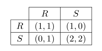
In generalized stag hunt, the agents are playing a game where there's a unique Pareto-optimal outcome. Under some not-too-restraining conditions, we expect the players to find this outcome. 

Conjecture: Suppose a set of players are playing a game with a unique Pareto-optimal outcome $a\in A$, and they follow the proposed algorithm. Suppose that for each player $i$, the hypothesis space $H_i$ consists of sharp infra-RDPs with at most $N_i$ number of states. Let $H_i^p=\{h\in H_i|h\text{is a password hypothesis}\}$. Suppose furthermore that $\exists \alpha :\underset{N_i\to \infty }{lim}\sum _{h\in H_p}{\zeta }_i\left(h\right)>\alpha$ for all $i$, and the length of the passwords is varying enough, then the agents will converge to the Pareto-optimal outcome with probability $1$ as $\underset{i}{max}{N}_i$ goes to infinity.

Reasoning behind the Conjecture:

• Suppose the agent starts to play assuming a hypothesis $h$. If $h$ will be falsified, how much time does it take falsify it? In theory, it could take any number of steps, but most of the time it should take more than $N_i$ steps. 
• Whenever an agent chooses a new hypothesis, it chooses a password hypothesis with probability at least $\alpha$. Thus, each agent is expected to try a new password hypothesis roughly every ${\alpha }^{-1}{N}_i$ steps.
• We can envision the learning process of agent $i$ as a random walk in $Z/\lceil {\alpha }^{-1}\underset{j}{max}{N}_j\rceil$. Let $\tau =\lceil {\alpha }^{-1}\underset{j}{max}{N}_j\rceil$. The first point of the random walk is the first time when the agent finishes entering a password in the first $\tau$ steps. The second point of the random walk is the first time when it finishes entering a password in steps $\tau +1,\dots ,2\tau$. If all the agents are at the same point of $Z/\tau$ at the same time, they have managed to reach the end of their password hypotheses at the same time and they will keep playing the Pareto optimal action.
• Will they reach the same point in their random walk before they run out of password hypotheses? There are $\Omega \left(2^{N_i}\right)$ password hypotheses for agent $i$ to try. If there are $k$ players, their combined random walk can be in ${\tau }^k$ states. If $N_i$ is big enough then $\Omega \left(2^{N_i}\right)$ is much bigger than ${\tau }^k$. If the lengths of the password hypotheses are varying enough, we can expect the agents to reach the same point before running out of hypotheses.

Prisoner's dilemma

In the Prisoner's dilemma, each agent gets the highest reward if they can exploit the other agent. That's also a very simple hypothesis, so it will be in the agents' hypothesis spaces. This means they will both start by defecting. Then each agent realizes their hypothesis was wrong, so they choose a new hypothesis. There can be differences based on the prior, but they will start by trying different hypotheses that let them get reward $3$ most of the time. Because both of them are trying to defect and expect the other to cooperate, they will falsify these ambitious hypotheses and start to cooperate for some of the time.

The figure below shows how the demands of the two agents might change in time. "Demand" here means what reward they can achieve based on the hypothesis they are currently assuming. The rational points inside the blue area are the realizable payoffs. They are realizable in the sense that there are hypotheses $h_1,h_2$ such that if agent $1$ plays assuming $h_1$ and agent $2$ plays assuming $h_2$, neither $h_1$ nor $h_2$ will be falsified. Conversely, the agents only have a chance of not falsifying their current hypotheses if they are inside the rhombus.

Remark: In general, the agents have a chance of not falsifying their current hypotheses if their demands are in the downward closure of the realizable payoffs.

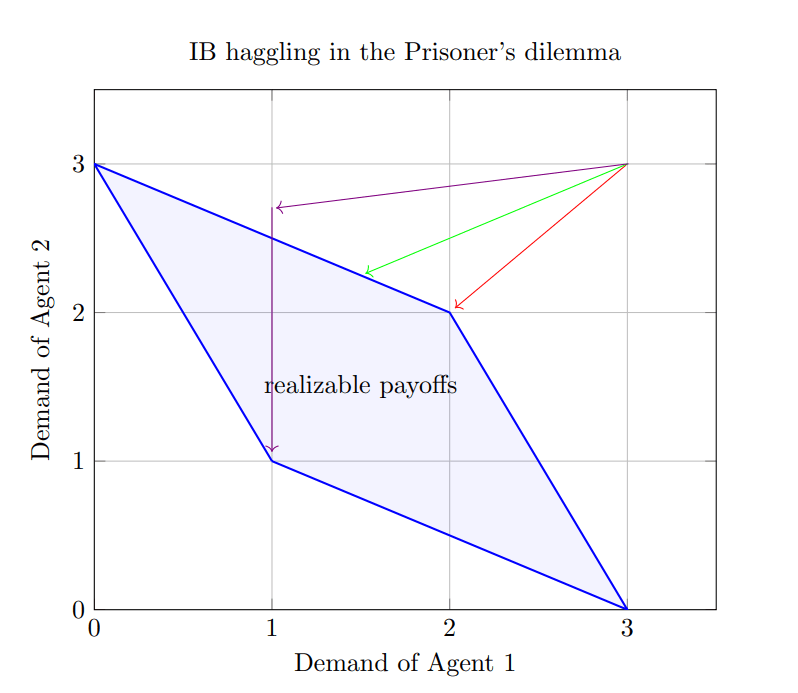
If the agents are similar enough, they will eventually reach a state where they are trying hypotheses that lets them play $(C,C)$ most of the time. If they have enough password hypotheses leading to $(C,C)$, it's plausible they will eventually start playing $(C,C)$ at the same time. (Red line.)

If agent 1 has slightly less of these ambitious hypotheses than agent $2$, they will probably converge to a behavior where they play $(C,C)$ some of the time and play $(C,D)$ otherwise. (Green line.)

If agent $1$ has a vastly different prior than agent $2$ and thus has much less ambitious hypotheses than agent $2$, then agent $1$ will lower its demand much faster than agent $2$. While trying hypotheses with utility $1$, Agent 1 will find a hypothesis that won't get falsified. The two agents can end up in $(1,1)$ or $(1,2.5)$ in this case. However, the more probable outcome is $(1,1)$, because $\top$ can't be falsified and it also has low complexity. (Violet line.)

Do the agents necessarily get into a stable cycle once they reach a realizable payoff? Suppose the agents reach a point of the blue rhombus: $(x,y)$. Let $H_x^p=\{h\in H_1|h\text{is a password hypothesis with utility}x\}$ and $H_y^p=\{h\in H_2|h\text{is a password hypothesis with utility}y\}$. If $H_x^p$ and $H_y^p$ are satisfying the conditions in the previous conjecture at that time, we can expect them to get into a stable cycle with payoff $(x,y)$. However, it is not clear if they would satisfy those conditions, even if they did so in the starting state. That's because the agents will have falsified some of these password hypotheses accidentally by the time they reach the rhombus. However, we could relax the definition of password hypotheses to allow more ambiguity, and hope that there are enough relaxed password hypotheses to reach a stable state. The idea is to allow slight deviations at the end-cycle of a password hypothesis that doesn't change the value of the hypothesis. For the password hypothesis below, there are two examples of a relaxed version. 

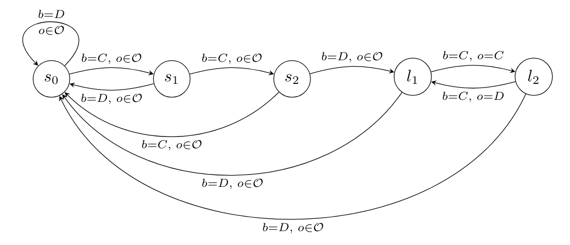
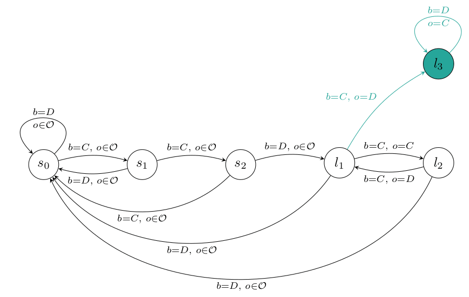
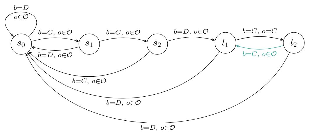
Another caveat here: in contrast to the stag hunt example, it is not enough if the agents reach the end of the password at the same time, they also need to have their cycle at the end of the password hypothesis in sync.

Conjecture: In a $2$-player game, the stable cycle will fall into one of the following cases:
1. Close to a Pareto-optimal outcome.
2. One of the agents gets the utility of its minimax strategy. The other player plays best response to the first agent's strategy.

Schelling Pub (Battle of the sexes)

In the Schelling Pub game [LW · GW] (a version of battle of the sexes), two friends would like to meet at the pub. They prefer different pubs, but both of them would rather be together in their unpreferred pub than sitting alone in their preferred pub.

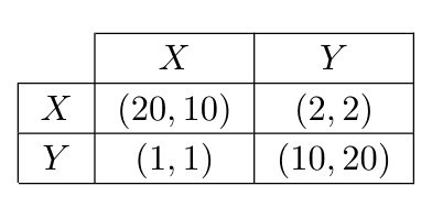
If the players are following our algorithm, they will reach a Pareto-optimal payoff: both going to pub $X$ for some of the time and both going to pub $Y$ otherwise.

An interesting thing to note. Suppose one of the players plays their minimax strategy, e.g. the person who prefers $X$, goes to $X$ no matter what. Then the other player will choose to go to the same pub and they will end up in a state that's better than what they would achieve if both of them played their minimax strategy. 

Schelling points

The Schelling Pub game is an example of people wanting to cooperate in a case where there are multiple options for cooperation. In that case, none of the possible cooperation states were more natural than the other. However, in some cases, there are points that are more natural targets of cooperation than others. These natural targets are called Schelling points [LW · GW].

Example: You ask three players to order the letters A, B, and C. If the three players give the same order, they win an award, otherwise they get nothing. Most players choose the ordering ABC. ABC is the Schelling-point in this game.

If IB agents are using the proposed algorithm and use a simplicity prior, simpler outcomes are more likely to arise as the result of haggling. In this way, haggling connects learning under a simplicity prior to reaching Schelling points.

Multiplayer games

If there are more than $2$ players, then players can form coalitions which makes things more difficult.

As always, players start with high demands. A set of players can form a coalition if they can guarantee the demanded payoff for each member of the coalition regardless of what strategy the players outside the coalition are playing. We can expect them to form a coalition in this case, and play the strategy that gives them the demanded payoff forever.

Note:  In the multiplayer case, Pareto efficiency is not guaranteed.

Example (Cake-splitting game): There are $3$ players. Each of them chooses another player they want to cooperate with. If two players choose each other, they will both get reward $\frac{5}{12}$, while the third player gets reward $0$. If there are no $2$ players who chose each other, everyone gets $\frac{1}{3}.$
In this case, the initial demanded payoff vector will be $(\frac{5}{12},\frac{5}{12},\frac{5}{12})$. Each player will try to get reward $\frac{5}{12}$ until two of the players manage to lock in and from that point on, the lucky players will have payoffs $\frac{5}{12},\frac{5}{12}$, while the third one will get $0$.
The interesting thing here is that "trying to cooperate with someone mutually" has expected utility $\frac{2}{3}\cdot \frac{5}{12}+\frac{1}{3}\cdot 0=\frac{5}{18}<\frac{1}{3}$, while "avoid mutual cooperation" has expected utility $\frac{1}{3}$. The reached payoff is Pareto-optimal, but the meta-strategy is not.

Example: There are $3$ players: Alice, Bob and Charlie. Each player can ask for reward $1$,  $2$ or $3$. If they ask for a payoff that's either $(3,3,1)$ or $(1,1,3)$, they get what they asked for. If it's $(2,2,x),$ then Alice and Bob get $2$, but Charlie gets $0.$ In other cases they all get $0$. They will start out with trying to get reward $3$. If they lower their demands at a similar rate, Alice and Bob will eventually ask for reward $2$ and that's where the haggling stops. This is not a Pareto-optimal outcome: they are getting payoff $(2,2,0)$, while they could get $(3,3,1)$ instead.

When can a coalition be formed?

It is not entirely clear. For a set of players $C\subseteq \{1,2\dots k\}$, let $U_C$ denote the set of payoff vectors they can certainly achieve without any assumptions on the strategies of players outside the coalition. A payoff vector $v$ is in $U_C$ if and only if there exists a probabilistic strategy of the coalition such that for any probabilistic strategy of the outsider players, each player $i$ in the coalition has expected reward at least $v_i$. Putting that together:

$U_C=\{v\in R^C|\exists \alpha \in \Delta \prod _{i\in C}{A}_i\forall \beta \in \Delta \prod _{i\in P\setminus C}{A}_i\forall i\in C:E_{\alpha \beta }[r_i]\ge v_i\}$

where $E_{\alpha \beta }\left[r_i\right]$ denotes the expected reward if members of the coalition choose a joint action sampling $\alpha$, while players outside the coalition choose their actions by sampling $\beta$.  $P$ denotes the set of players.

This definition of $U_C$ assumes the randomness used in the strategies isn't shared between the coalition and the outsiders. Is this a realistic assumption?

At first glance, this is not the case with sharp infra-RDPs. Once an agent chooses a hypothesis, it follows a deterministic policy until the hypothesis is falsified. Mixed stage strategies are encoded in deterministic cycles, like the loops in password hypotheses.

It is possible that more sophisticated learning algorithms could come up with some kind of cryptographic solution to form a coalition whenever the payoff vector is in $U_C$. However, for the algorithm proposed in this post, this is not the right criterion for forming coalitions.

Next, we give a definition of $U_C^{\prime }$ that allows the outsiders to sync their actions with the actions of the coalition members.

$U_C^{\prime }=\{v\in R^C|\exists {\alpha }_c\in \Delta \prod _{i\in C}{A}_i\forall \alpha \in \Delta A:\text{if}\alpha {|}_C={\alpha }_c\text{, then}\forall i\in C{E}_{\alpha \beta }[r_i]\ge v_i\}$

where $\alpha {|}_C$ denotes the distribution we get by marginalizing $\alpha$ to $\prod _{i\in C}{A}_i$.

Stable cycles for multiplayer games

Where will haggling lead in this case? Once there is a coalition $C$ such that the current demanded payoff vector $v$ is in $U_C^{\prime }$, players in $C$ can lock in on a strategy that guarantees $v$. From that point on, outsiders can only keep a hypothesis unfalsified if it's consistent with $C$'s locked strategy.

If $C_1\dots C_m$ has been formed, a new coalition $C_{m+1}$ will be formed if the players in $C_{m+1}$  can guarantee their demanded payoff assuming the players in $\bigcup _{j=1}^m{C}_j$ are playing their locked strategy.

Let $C_{\le m}=\bigcup _{j=1}^m{C}_j$ be the set of players already in a coalition. Let ${\alpha }_{\le m}\in \Delta \prod _{p\in C_{\le m}}{A}_p$ be the strategy played by members of $C_{\le m}$. Now a set of players C can choose from strategies in $C_{strategy}=\{\alpha \in \Delta \prod _{i\in C_{\le m}\cup C}{A}_i:\alpha {|}_{C_{\le m}}={\alpha }_{\le m}\}$. The payoff vectors $C$ can achieve are

$U_{C,{\alpha }_{\le m}}^{\prime }=\{v\in R^C|\exists {\alpha }_c\in C_{strategy}\forall \alpha \in \Delta A:\text{if}\alpha {|}_C={\alpha }_c\text{, then}\forall i\in C{E}_{\alpha \beta }[r_i]\ge v_i\}$

How we expect a stable cycle to look like? The players form coalitions $C_1,C_2\dots C_n$ such that it's a partition of the players.  Let $v\in R^k$ be the payoff vector they reached. Then for each $m$

• the payoff of $C_m$'s members is in $U_{C_m,{\alpha }_{\le m-1}}^{\prime }$
• there does not exist any set of players $C^{\prime }\subseteq C_m$, such that there exists $v^{\prime }\in U_{C^{\prime },\le {\alpha }_{m-1}}^{\prime }$ with $v_i<v_i^{\prime }$ for each $i\in C^{\prime }$. Otherwise $C^{\prime }$ would have been formed instead of $C_m$.

Conclusion

We have described a natural infra-Bayesian learning algorithm and investigated its behavior in different repeated games. We have shown informally why we expect this algorithm to often find Pareto-optimal outcomes in two-player games. We also looked into its connection to Schelling points. Finally, we explored the states IB agents can reach in multiplayer games where coalitions can be formed.

Future directions

• Formally prove the conjectures mentioned in the post.
• Generalize this algorithm to a stochastic setting for all resettable infra-RDPs. 
• For a countable hypothesis set $H$, we defined finite sets $H_{\gamma }$, such that if the true environment satisfies $h\in H$, and the prior over the hypotheses assigns a positive weight to $h$, then the proposed algorithm ${\pi }_i^{\gamma }$ ensures$\underset{\gamma \to 1}{lim}\underset{{\pi }_{-i}\in {\Pi }_{-i}^h}{min}{u}_i({\pi }_i^{\gamma },{\pi }_{-i},\gamma )\ge \underset{\gamma \to 1}{lim}{V}_i(h,\gamma )$. Possibly, the algorithm can be modified in a way that instead of a separate policy for each $\gamma$, we can define one policy ${\pi }_i$ that ensures $\underset{\gamma \to 1}{lim}\underset{{\pi }_{-i}\in {\Pi }_{-i}^h}{min}{u}_i({\pi }_i^{}{\pi }_{-i},\gamma )\ge \underset{\gamma \to 1}{lim}{V}_i(h,\gamma )$. We say the hypothesis set $H$ is anytime-learnable in that case. This would require to extend the set of hypotheses considered over time. One difference in principle is, even if the players started playing some Pareto-optimal sequence, each of them would occasionally deviate from it to try for a higher payoff, potentially falsifying the hypotheses of the other players. Hopefully, after every such deviation, the players will eventually settle back using the same mechanism. This would "burn" some passwords, but also new (longer) passwords would enter consideration over time.
• What is the broadest natural category of infra-Bayesian learning algorithms with such convergence guarantees?
• Instead of a repeated game, we can consider a population game where each agent has access to the internal state of its opponents at the start of the round (in particular, the history they experienced). Getting Pareto-optimality there requires some new idea: since each agent faces new opponents on each round, there is no longer "lock-in" of a Pareto-optimal outcome. Possibly, we would need to consider a family of hypotheses which postulate progressively higher portions of the population to be cooperative.

Appendix

Proof of Proposition 1: Fix a copolicy ${\pi }_{-i}$. Let $N=\underset{h_j\in H}{max}\left\{|S_{h_j}|\right\}$. For action $b$ and observation $o$, let $r_i(b,o)$ denote the reward the agent receives after playing action $b$ and observing $o$. Let $R=\underset{h_j\in H_i;(b_1,o_1),(b_2,o_2)\in A_{h_j}\times O_{h_j}}{max}\left\{r_i\right(b_1,o_1)-r_i(b_2,o_2\left)\right\}$ be the maximal possible regret. Suppose the agent follows the proposed algorithm ${\pi }_i$ and tries hypotheses $h_1\dots h_F$, falsifies them, and eventually reaches $h_{F+1}$ that remains unfalsified. For $j\le F$, let $f_j$ denote the time step when the agent falsifies $h_j$.

Let us call a series of at least $2$ consecutive steps that starts and ends in the same state a cycle. A path is any series of consecutive steps. Let $f_j=0.$ For each $j\le F$, we will partition the steps between $f_{j-1}$ and $f_j$ into paths and cycles using the states of hypothesis $h_j$. $h_j$ is a false hypothesis, but during those steps, the world is consistent with $h_j$, so we can use its states to reason about these steps. We define the cycles using the following algorithm. Let $s_1^j\in H_j$ be the state the agent is at step $f_{j-1}+1$. If the agent returns to $s_1^j$ before step $f_j$, let the first cycle consist of the steps between step $f_{j-1}+1$ and the last occurrence of  $s_1^j$. Now let $s_2^j\in H_j$ be the state after the last occurrence of $s_1^j$. If it appears again before step $f_j$, then let that be a cycle, and so on. The paths are the steps connecting two cycles. Using this, we will partition the time steps into $3$ groups:

$N_1=\{n:\text{step}n\text{is in a path or it is the last element of a cycle}\}\cup \{f_1\dots f_F\}$
$N_2=\{n:\text{step}n\text{is in a cycle, but not the last step of the cycle}\}$
$N_3=\{n:n>f_F\}$

Based on which group $n$ belongs to, we will use different lower bounds of the weighted reward at step $n$.

For $n\in N_1$, we will use the lower bound $r_i\left(a^{\left(n\right)}\right)\ge V_i(h,\gamma )-R$. Note $|N_1|\le |H|(N+1)$. Hence

$(1-\gamma )\sum _{n\in N_1}{\gamma }^n{r}_i\left(a^{\left(n\right)}\right)\ge (1-\gamma )\sum _{n\in N_1}{\gamma }^n{V}_i(h,\gamma )-(1-\gamma )|H|(N+1)R$

Before we get into the lower bounds for steps in $N_2$, let us introduce a new notation. For hypothesis $h_j$, let us define a slightly modified version of it, $h_j^s.$ The only difference is the start state: the start state in $h_j^s$ is $s$. $V_i(h_j^s,\gamma )$ can be different than $V_i(h_j,\gamma )$. However, it can't be much lower. Because $h_j$ is resettable, the agent can get to $s_0$ in at most $N$ steps and play the policy that ensures utility $V_i(h_j,\gamma )$ from that point on. Thus $V_i(h_j^s,\gamma )\ge V_i(h_j,\gamma )-(1-\gamma )NR$.

To give a lower bound for steps in $N_2$, let $x$ and $y$ denote the start and end of a cycle. Suppose this is a cycle between $f_{j-1}$ and $f_j$. We would like to use $V_i(h_j,\gamma )\ge V_i(h,\gamma )$ to give a lower bound on the weighted sum of rewards between steps $x$ and $y$. Let ${\pi }_{-i}^{\prime }$ denote the copolicy that is the same as ${\pi }_{-i}$ until step $y$, then repeats the observations between $x$ and $y$ infinitely. Let $s_x\in S_j$ be the state at time step $x$. Then

$\begin{array}{cc}{V}_i(h_j,\gamma )& \le V_i(h_j^{s_x},\gamma )+(1-\gamma )NR\\ & \le (1-\gamma )\left(\sum _{c=0}^{\infty }{\gamma }^{c(y-x)}\sum _{n=0}^{y-x-1}{\gamma }^n{r}_i\right(a^{(x+n)}\left)\right)+(1-\gamma )NR\end{array}$

With the notation $U=(1-\gamma )\sum _{n=0}^{y-x-1}{\gamma }^n{r}_i\left(a^{(x+n)}\right)$:

$\begin{array}{cc}{V}_i(h_j,\gamma )& \le \frac{U}{1-{\gamma }^{y-x}}+(1-\gamma )NR\\ V_i(h_j,\gamma )& \le \frac{{\gamma }^{x}U}{{\gamma }^x-{\gamma }^y}+(1-\gamma )NR\\ ({\gamma }^x-{\gamma }^y)V_i(h_j,\gamma )-({\gamma }^x-{\gamma }^y)(1-\gamma )NR& \le {\gamma }^{x}U\\ ({\gamma }^x-{\gamma }^y)V_i(h,\gamma )-(1-\gamma )NR& \le {\gamma }^{x}U\end{array}$

Using $\sum _{n=x}^{y-1}{\gamma }^n=\frac{{\gamma }^x-{\gamma }^y}{1-\gamma }$, we get

$\begin{array}{cc}(1-\gamma )\sum _{n=x}^{y-1}{\gamma }^n{r}_i\left(a^{\left(n\right)}\right)& ={\gamma }^{x}U\\ & \ge ({\gamma }^x-{\gamma }^y)V_i(h,\gamma )-(1-\gamma )NR\\ & \ge (1-\gamma )\sum _{n=x}^{y-1}{\gamma }^n{V}_i(h,\gamma )-(1-\gamma )NR\end{array}$

The number of cycles in our partition is at most $N|H|$, hence

$(1-\gamma )\sum _{n\in N_2}{\gamma }^n{r}_i\left(a^{\left(n\right)}\right)\ge (1-\gamma )\sum _{n\in N_2}{\gamma }^{n}V(h,\gamma )-(1-\gamma )|H|N^{2}R$

Finally, for steps in $N_3$, we have

$(1-\gamma )\sum _{n=f_F}^{\infty }{\gamma }^n{r}_i\left(a^{\left(n\right)}\right)\ge (1-\gamma )\sum _{n=f_F}^{\infty }{\gamma }^{n}V(h,\gamma )-(1-\gamma )NR$

Putting the bounds for $N_1,N_2$ and $N_3$ together, we get

$\begin{array}{cc}u({\pi }_i,{\pi }_{-i},\gamma )& =(1-\gamma )\sum _{n=0}^{\infty }{\gamma }^n{r}_i\left(a^{\left(n\right)}\right)\\ & \ge (1-\gamma )\sum _{n=0}^{\infty }{\gamma }^n{V}_i(h,\gamma )-(1-\gamma )3|H|N^{2}R\\ & =V_i(h,\gamma )-(1-\gamma )3|H|N^{2}R\\ \underset{\gamma \to 1}{lim}u({\pi }_i,{\pi }_{-i},\gamma )& =\underset{\gamma \to 1}{lim}{V}_i(h,\gamma )\end{array}$
 

0 comments

Comments sorted by top scores.