LLM Modularity: The Separability of Capabilities in Large Language Models

post by NickyP (Nicky) · 2023-03-26T21:57:03.445Z · LW · GW · 3 comments

Contents

  TL;DR
  5 Minute Non-Techincal Summary
  Full Technical Report
  1. Introduction
    1.1 Relevant Literature
  2. Method
    2.1. Models Used – Meta OPT and Galactica
    2.2. Task Separability
      2.2.1. Tasks Used – Pile, Code and Python 
      2.2.2. Task Definition
      2.2.3. Task Extraction
      2.2.4. Task Metrics of Performance
    2.3. Separability Measurement
      2.3.1. Pruning Trajectories
        Random Pruning Trajectory
        Selective Pruning Trajectory
      2.3.2. Separability Areas
      2.3.3. Separability Area Percentages
    2.4. Pruning Procedure
      2.4.1. Feed Forward Block Pruning
      2.4.2. Attention Pruning
        Pruning Attention with SVD
        Pruning Attention Heads
      2.4.3. Random Removal
      2.4.4. Summary of Pruning Options
        Feed Forward Pruning:
        Attention Pruning:
  3. Results
    3.1. Choosing the Best Pruning Method
      3.1.1 Pruning Galactica 1.3b
      3.1.2. Pruning OPT 1.3b
      3.1.3 Bi-Directional Pruning - FF Only
      3.1.3 Bi-Directional Pruning - ATTN Only
    3.2. Pile vs. Code Separability in Meta's Models
    3.3. Code vs. Python Separability in Meta's Models
    3.4 Civil Comments
    3.5. Other Observations
      3.5.1 "Backup" Mechanisms
      3.5.2 Threshold Spikes
      3.5.3 Late-Pruning Performance Jumps
    3.6. Limitations
  4. Understanding What is Happening
    4.1. Attention vs. MLP
    4.2 The Basis of Computation Might Be Neuron-Aligned
      4.2.1 The "Curse of Dimensionality" means that most vectors are almost orthogonal
      4.2.1 SVD can be disrupted by noise
    4.3. Further Work
  5. Conclusion
  6. References
  Appendix A: Choosing Scoring Functions for Attention Neuron Distributions
      Some examples of distributions
None
3 comments

Post format: First, a 30-second TL;DR, next a 5-minute summary, and finally the full ~40-minute full length technical report.

Special thanks to Lucius Bushnaq for inspiring this work [AF · GW] with his work on modularity [AF · GW].

TL;DR

One important aspect of Modularity, is that there are different components of the neural network that are preforming distinct, separate tasks. I call this the “separability” of capabilities in a neural network, and attempt to gain empirical insight into current models. 

The main task I chose, was to attempt to prune a Large Language Model (LLM) such that it retains all abilities, except the ability to code (and vice versa). I have had some success in separating out the different capabilities of the LLMs (up to approx 65-75% separability), and have some evidence to suggest that larger LLMs might be somewhat separable in capabilities with only basic pruning methods.

My current understanding from this work, is that attention heads are more task-general, and feed-forward layers are more task-specific. There is, however, still room for better separability techniques and/or to train LLMs to be more separable in the first place.

My future focus, is to try to understand how anything along the lines of "goal" formation occurs in language models, and I think this research has been a step towards this understanding.

 

5 Minute Non-Techincal Summary

I am currently interested in understanding the "modularity" of Large Language Models (LLMs). Modularity is an important concept for designing systems with interchangeable parts, which could lead to us being better able to do goal alignment for these models.

In this research, I studied the idea of "Separability" in LLMs, which looks at how different parts of a system handle specific tasks. To do this, I created a method that involved finding model parts responsible for certain tasks, removing these parts, and then checking the model's remaining capabilities.

There are a few papers that have been looking at related things, which I try to briefly summarise. Most have been related to trying to build "modular" language models, in the sense of trying to build models where you can run only a fraction of the neurons to save computation time.

There have also been a small number of papers that retrofit a normal language model into these more "modular" architectures (in the style of "Mixture of Experts"), and have some interesting results. One limitation, is that these have only focused on feed-forward layers in LLMs, and have neglected trying to understand attention layers.

 

To examine task separability, I used Meta's OPT and Meta's Galactica to look at next-token prediction on three datasets as proxies for general tasks. 

The datasets I used were:

• Pile (general text)
• Code (various programming languages from GitHub)
• Python (a subset of Code containing only Python code).

I then compared Pile vs. Code and Code vs. Python.

I used two procedures to separate tasks from a language model, one focused on removing specific capabilities and the other on removing general tasks. I pruned neurons in the models in the Feed Forward mid layers, and the Attention Heads by comparing activation statistics for each neuron between the two tasks. I used different accuracy measures based on next-token prediction in the datasets to evaluate the performance.

In my study, I used various pruning methods to remove task capabilities from the models. I focused on pruning the MLP and Attention blocks and compared neuron activations across different datasets. I also used random removal as a baseline.

To visualise task separability, I plotted the performance in one task against another and used the area under the curve as a proxy for separability. Although this metric has limitations, it is perhaps a useful starting point.

I analysed the results for Pile vs. Code and found that pruning Feed Forward layers worked well, while pruning Attention layers was more difficult but still okay. Larger models seemed to show somewhat more modularity (up to approx 65-75% separability) compared to smaller models (approx 45-65% separability).

I then looked at a more challenging scenario: separating Python coding ability from general coding ability, and effectiveness was limited. Here, model size had a huge effect on separability, where smaller models where approx 0-20% modular, and larger models were approx 20-35% separable.

My research findings slightly suggest that the MLP layers in transformers are more task-specific, while the attention heads appear to be more task-general.

One interesting observation was that performance sometimes increasing instead of decreasing after several pruning steps.

Despite the promising results, there is still much to be done in understanding the modularity of large language models. Future research should include conducting experiments with fine-tuning instead of pruning, investigating more meaningful performance metrics, optimising pruning parameters, and exploring better pruning methods for attention heads.

The are likely many methodological flaws here, but as there are so many research directions I could pursue from here (about 15, listed in "4.3. Further Work"), I have decided to publish the current state of my research for now. I have listed some possible further investigations in my work.

I plan to work further in this direction, and would like to attempt to separate out "Tasks" vs "Goals" in whatever way this might be possible, and hope to eventually understand what "long term goals" might look like in language models (or the simulacra that they simulate). This be feasible in current LLMs, or it might require adjusting LLM training to induce more separability.

I welcome feedback from anyone on better metrics and methodologies to improve our understanding of separability in Large Language Models. If anyone wants to work on any of these questions, or has suggestions on what they would like to see most, I am open to people reaching out to me.

Full Technical Report

1. Introduction

I am interested in the way that a Large Language Model (LLM) might have different parts dedicated to doing different general tasks. While I’m not sure if LLMs in their current form could build an AGI capable of advanced research, it is likely that some aspects of their architectures, such as attention heads and residual streams, might play key parts in a future AGI.

One of the key desiderata of modularity would be to have the capability to extract modules from various systems, to such a degree that one could mix and match them with each other. In particular, if there is a modular part of a model dedicated to having a goal, then one could give the model the best goal.

In this research, I have been trying to investigate any possible way we might consider modularity in LLMs. Though there have been attempts with MLP networks to attempt to define modularity in terms of the graph structure of the model (Filan 2020; Bushaq 2022), this ontology does not naturally continue to LLMs. It is also likely that there have been key mistakes with how I am attempting to consider modularity and how it generalised to other models, but I will be attempting anyway.

While modularity bring to mind many things to different people, one important property is what I will call “Separability”, which is sometimes called "degree of task specialisation" in the literature.

Separability: The extent to which there are different "parts" of a system that are separately and uniquely responsible for computing different tasks.

My current method, is to consider two sets of tasks. I attempt to identify parts of the model that are responsible for doing one set of tasks, and ablating them, such that the model is no longer able to do that set of tasks, is still capable in the other set of tasks. My current method for identifying these parts are quite primitive and clunky, and likely only intervenes at one part of the process of the task rather than the whole process (i.e: only part of a circuit, and not the whole circuit). Nevertheless, I have still managed to show at least some progress in the task separability for both Feed Forward and Attention layers.

I tried to focus on relatively quite general tasks (like coding) rather than more specific tasks with easily known answers, but this is limited since I was still using next-token prediction as the task in my current research. I would ideally like to find more general parts of the model (that are less "specific tasks" and more "longer-term goals", which eventually steer the direction of outputs a model can make), but this will be left to future research. 

I would like to eventually be able to understand how one can distinguish "tasks" and "goals" in language models, and while I have not yet made direct progress on this yet, I think I have gained some intuitions on how this might happen from this research.

1.1 Relevant Literature

I mostly tried to do this research without getting biases by current methods, though have recently reviewed some of the recent literature on modularity in language models, and found that there is some overlapping work. 

Most modularity work is focused on improving capabilities with a smaller compute budget. For an overview of such approaches, see the recent paper "Modular Deep Learning".

Some of the most relevant papers have been by Zhengyan Zhang et. al, including their paper on "Moefication: Transformer feed-forward layers are mixtures of experts". This paper looks at trying to group Feed Forward neurons into clusters/groups of "experts" (following the Mixture of Experts paradigm), and add a "routing" function to only activate the most likely useful fraction of feed forward neurons. I think this is a useful paper, and shows a gives good information on the separability of capabilities in Feed Forward layers

In a more recent paper "Emergent Modularity in Pre-trained Transformers", they looked at feed forward layers, and attempted to measure modularity in them. They looked at neuron-by-neuron scores as well as used "MoEfication" to cluster neurons into Mixture of Expert (MoE). This is pretty relevant and has a lot of overlap with my current research, and is a good paper. I think my research still provides some valuable information from a different perspective, particularly when looking at Attention neurons.

One particular finding from the paper and some referenced papers that I have not yet read, is that although you can try to build an LLM to be modular (eg: by a huge number of different ways described in "Modular Deep Learning"), the simplest ("non-modular") models seem to be more "modular". Though this was only on quite rough modularity metrics tested, this matches my intuitions.

Lastly, are papers like "Are Sixteen Heads Really Better than One?", which look at trying to prune unused attention heads without affecting performance. My research is does want to affect performance, but only differentially on some tasks. In addition, I also look at on the scale of attention neurons instead of only on the scale of attention heads.

 

In a different recent paper "Editing Models with Task Arithmetic", the authors tried to edit models to do (or not do) certain tasks by fine-tuning the model on the task, and using the difference in parameters as a vector. The negating vector example they used, was generation of toxic comments by fine-tuning the model on the task, then negating the difference in weights. While this captures some of what I am interested in, I would prefer methods where this isn't needed (as for AGI, this would involve fine-tuning it to be super evil, which for some kinds of models is already catastrophic). I quickly adapted my pruning technique to do the same and it was similarly successful.

A paper that is somewhat tangentially related is "Discovering Latent Knowledge in Language Models Without Supervision", which is like a different approach to influencing the outputs of a Language Model by adjusting the latent space directly. I think my research is somewhat different to this approach, but has a somewhat similar goal.

Another tangentially related paper released a couple weeks ago is "Eliciting Latent Predictions from Transformers with the Tuned Lens", which I may try to integrate into my research, but I have not yet.

 

2. Method

2.1. Models Used – Meta OPT and Galactica

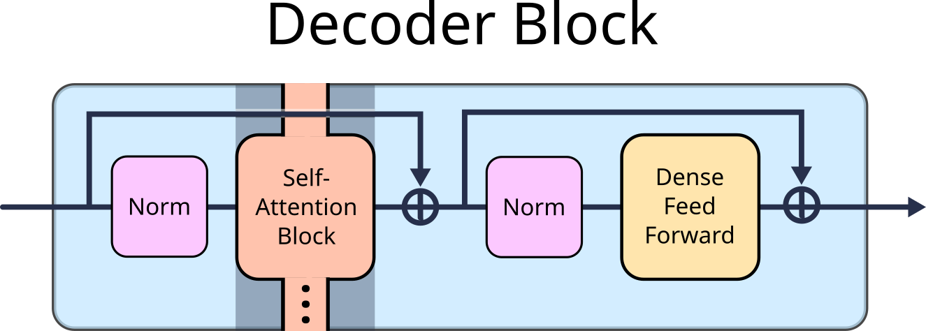
So far, the models I have been looking at, are Meta’s OPT and Galactica models in various sizes. Both are have what could be considered the standard decoder structure for a decoder-only large language models. Some of the main relevant differences are:

OPT models are:

• Trained on the Pile.
• Use ReLU activation function.
• Have all the normal biases.
• Use the GPT2 tokeniser.

Galactica models are:

• Trained on a dataset of mostly papers.
• Use GeLU activation function.
• Does not use biases in any of the dense kernels or layer norms
• Use a custom-trained tokeniser.

 

2.2. Task Separability

2.2.1. Tasks Used – Pile, Code and Python 

As proxies for types of general tasks, I have used next-token prediction on “Pile”, “Code” and “Python” datasets, which are:

• “Pile”: ElutherAI The Pile Deduplicated
  • A general text dataset, that includes some amount of code (approx 10%)
• “Code”: CodeParrot GitHub Code (all-all)
  • A code dataset of various different languages on GitHub
• “Python”: CodeParrot GitHub Code (python-all)
  • The subset of the previous dataset that only contains python code

I also briefly used the "civil comments" dataset, which I have split into two parts:

• "Civil": Civil Comments Low Toxicity (<0.2)
• "Toxic": Civil Comments High Toxicity (>0.8)

For collecting activations, I would collect a sample of 100,000 next-token predictions. For doing evaluations, I would collect enough tokens such that one I remove "skipped tokens" (see below) I would have a sample of 100,000 "non-skipped" tokens. I have found larger samples to work somewhat better, but at the trade-off of being significantly slower, and found ${10}^5$ was a decent compromise (a sample of approx 100 texts). 

 

 

2.2.2. Task Definition

We consider how we can separate out tasks. We consider a “general” task which has two subsets of tasks:

• The “specific” sub-task we are considering
• The “remaining” sub-tasks (which are part of the “general” task but not of the “specific” task)

The pairs of General & Specific task I have been using, are:

• Pile & Code
• Code & Python

In current models, it seems likely that there are components that can be classified on some continuum as:

1. Useful for the specific sub-task.
2. Useful for both the specific and remaining sub-tasks of the general tasks.
3. Useful for the remaining sub-tasks of the general task.

 

2.2.3. Task Extraction

We accept that there are multiple ways one can attempt to extract task performance. I will mostly assume that when extracting a task, that we are removing capabilities from a model, and propose that there are two procedures one could consider when separating out different tasks from a language model. These are:

• To remove specific capabilities from a model, and keep remaining general tasks.
• To remove all remaining general tasks, and keep only the specific task.

These procedures shall be called "specific cripple" and "specific focus" tasks respectively. That is, for the pairs of tasks we are looking at, we could say:

• For Pile & Code, we will do a “code cripple” and “code focus” procedure.
• For Code & Python, we will do a “python cripple” and “python focus” procedure.

By comparing the performance of the model on both, one can evaluate how well one could focus in on specific capabilities of the model.

 

2.2.4. Task Metrics of Performance

The metrics of performance I have been using are related to prediction accuracy, (instead of using loss directly):

• % Top1 Next Token Prediction Accuracy
• % Top10 Next Token Prediction Accuracy
• % Skip50 Top1 Token Prediction Accuracy
• % Skip50 Top10 Token Prediction Accuracy

Here, Skip50 refers to ignoring token predictions if the token being predicted is one of the 50 most common possible tokens in the dataset. I haven’t "skip" metrics like this used elsewhere, but it seemed like a potentially useful metric for measuring slightly more interesting parts of performance.

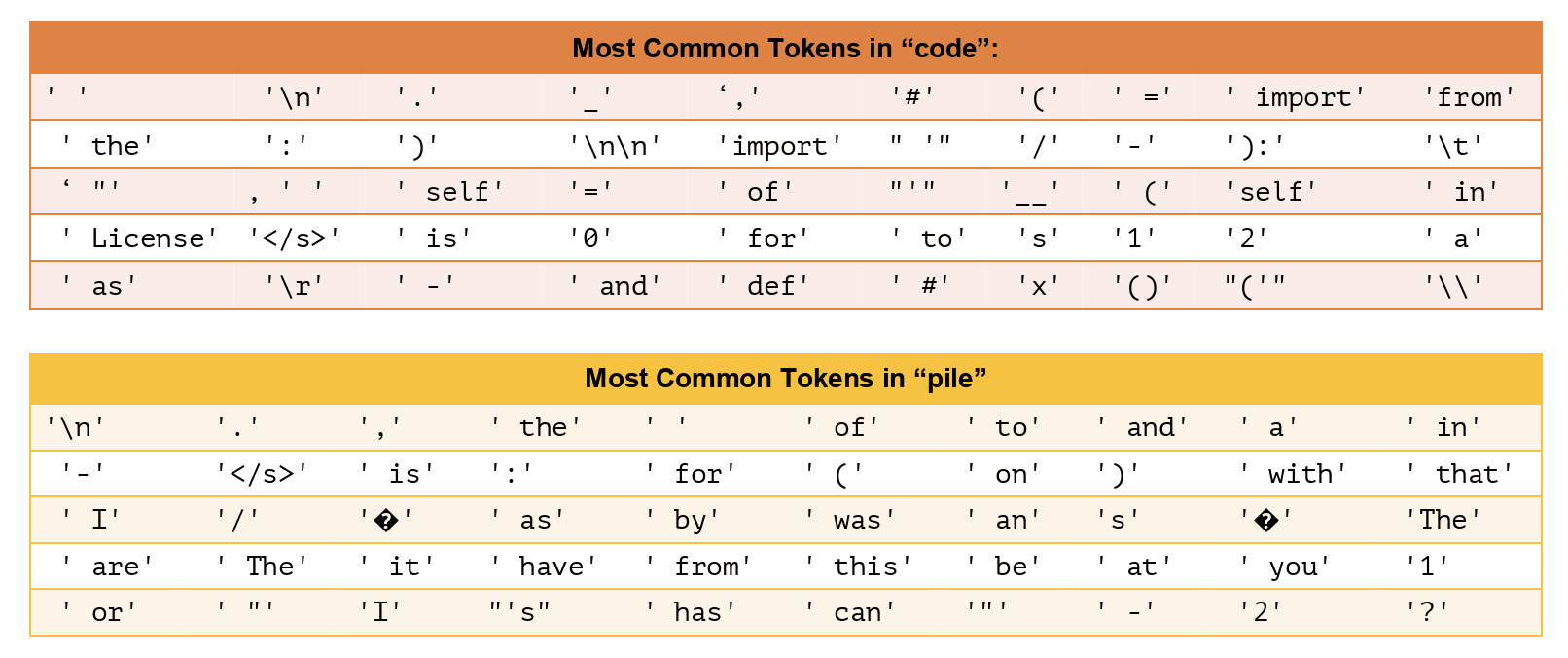
It seems plausible that we don't really care that much about how good the model is at predicting these accurately, since it represents the "easy" part of next token prediction. I found that looking at these can give a slightly better picture as to what is happening in the pruning process. 

Note: One methodological error I made, is that I changed datasets to similar alternatives after calculating these most common tokens, and did not recompute the most common tokens, so these will not be completely accurate. I should probably have re-run the experiment evaluations. I believe that the results are still qualitatively accurate.

 

2.3. Separability Measurement

2.3.1. Pruning Trajectories

Since we are pruning iteratively (described in the next section), one way to visualise the performance of different methods, one can compare the metrics of performance in different tasks. In particular, one can plot on two axes, the performance in one task against the performance in another task. We call this a "pruning trajectory".

We can compare the pruning to a random baseline, and get a visual intuition on how separable the pruning is, and where there might be limitations to the separability.

The following is a fictional example of a pruning trajectory, for the example of code vs pile, where here we are trying to selectively cripple code performance:

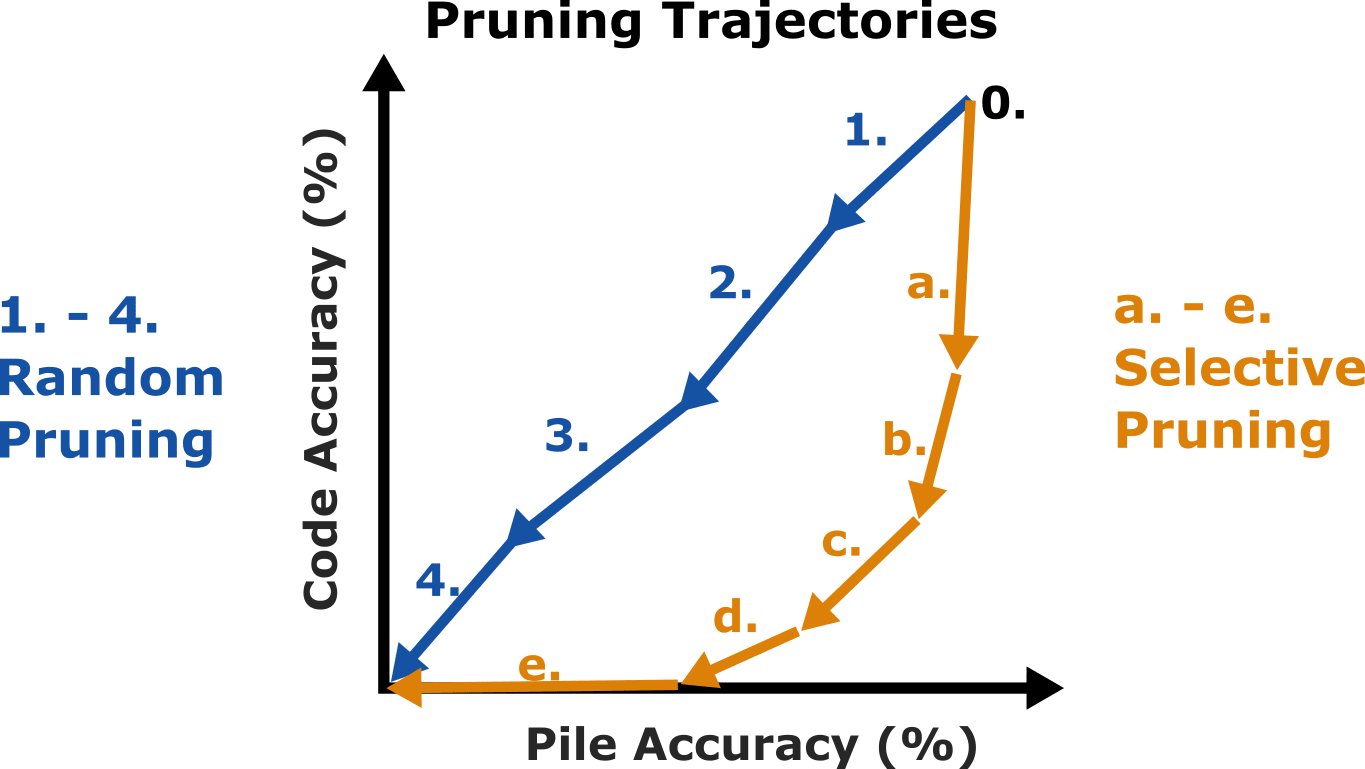
Here is an idealised story of what is happening in this fictional graph for both the random and selective pruning trajectories:

(0). We start off with an evaluation (on both tasks) of the unpruned models. Thus, they are seen as starting at the same point on the pruning trajectories.

Random Pruning Trajectory (1). We prune the model randomly by some amount, and evaluate the new performance. We see a moderate drop in code performance We see a moderate drop in pile performance As a result, we see our new evaluation is an almost diagonal line down from the original evaluation, since there was no differential effect between pruning code and non-code neurons.   (2). We prune the remaining neurons randomly by some amount, and evaluate performance again. We see a moderate drop in code performance We see a moderate drop in pile performance Our new evaluation point is again almost diagonally down from the previous point, similar to before   (3). We, again prune randomly and evaluate. We see a moderate drop in coding performance We see a moderate drop in pile performance Our new evaluation point is again almost diagonally down from the previous point.   (4). We prune randomly and evaluate one last time. We see a moderate drop in coding performance We see a moderate drop in pile performance Our new evaluation point is again almost diagonally down from the previous point.  Performance is now at almost zero at both tasks, since we have deleted so many neurons the model is no longer able to make accurate predictions for either the pile or for code.

Selective Pruning Trajectory (a). We prune the model selectively by some amount, and evaluate the new performance. We see a large drop in code performance We see a tiny drop in pile performance As a result, we see our new evaluation is an almost vertical line down from the original evaluation, since we have mostly only neurons that were mostly only used for "coding".   (b). We prune the remaining neurons selectively by some amount, and evaluate performance again. We see a moderate drop in code performance We see a small drop in pile performance Our new evaluation is a less steep vertical line down, that goes to the left more than last time. The neurons we just pruned are still mostly only for code, but are partially useful for pile too.   (c). We prune selectively again....   (d). We try again to prune selectively and evaluate. We see a small drop in code performance to almost zero. We see a larger drop in pile performance As almost all the coding performance is already gone, so we end up mainly pruning pile neurons that are sometimes useful for code. The model has zero code performance by the metric being used.   (e). We try again to prune selectively, and evaluate We see a almost no drop in code performance (already close to zero) Pile performance now goes down to almost zero. Our new evaluation shows the mode is no longer able to make any accurate predictions. The step from the previous point is an almost horizontal line to zero.

Note that we could also be doing "code focus" instead of "code cripple", in which case we will get a pruning trajectory that is similarly shaped, but mirrored about the diagonal. We look at the pruning trajectories for the different metrics, and the exact story does not always follow the stories written above, but there is at least some truth to the above stories.

 

2.3.2. Separability Areas

Now that (hopefully) we understand how the pruning trajectories work, we can invent a summary metric that captures some of the information captures in the pruning trajectories.

We can gain intuition on how “modular” the model might be. We look at some examples of possible pruning trajectories.

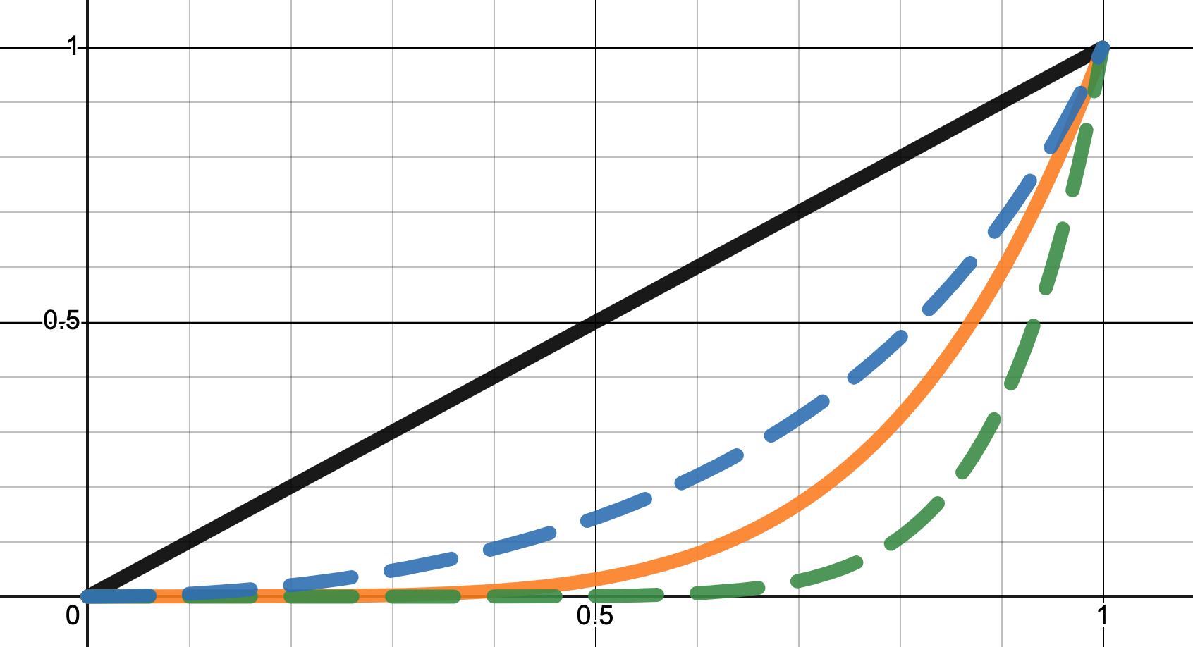
We see that the more diagonal the line, the less "separability" the pruning trajectory shows.

Somewhat inspired by inequality measures, one can look at the area under the curve as more of the model gets pruned. Initially, the model begins in the upper right corner, where Specific and General task performance is high. Then, after a step of pruning, we will get a point that is slightly lower performance at both the specific and general task. We can repeat this procedure iteratively until the whole model is pruned.

In this case, the more close the curve is to a straight line, the worse we are able to separate out the performance on the two tasks. The closer the curve is to a rectangle, the more we are able to separate out the performance on the two separate tasks. We can compute a summary of how good a job we did at separating out the tasks, by calculating the area under the curve. Then:

• Area=0.0 corresponds to perfect separability towards one task.
• Area=1.0 corresponds to no separability.
• Area=2.0 corresponds to perfect separability towards the other task.

This is a flawed metric, but I think might be a useful as a proxy for separability in this case. In particular, some flaws are:

• It makes it seem like separability is linear to this metric (e.g: a score of 0.5 means it is 50% modular, or that 0.9 means it is 10% modular). It might be however that a score of 0.1 is more like 1% modular, or more like 30% modular. I have no idea which it is
• It does not particularly focus on the most important part of the separability, which I think is likely going to be within the regime of little performance loss.

 

2.3.3. Separability Area Percentages

The above explanation on pruning trajectories and pruning areas are difficult to explain quickly, and it can be useful to have something in a format that is more easy to understand. For this reason, I think it is useful to have a metric of separability that could said quickly to give a rough idea on results. I think that deviation from 1.0 (to either 0.0 or 2.0) can quickly give a better impression on separability. 

To (hopefully) reduce confusion, I propose a "separability percentage" based on the separability area score, which is just $100\times |1-\text{area}|$. That is, as separability area of 0.3 or of 1.7 would both give 70% separability. This might be somewhat misleading, since the "area" separability score is not necessarily linear in an ideal metric of modularity, but I err on the side of this being fine.

A better metric might not so much measure deviation from 1.0, but instead be normalised to how well random pruning works. I will use unnormalised separability area percentages for now.

 

2.4. Pruning Procedure

While in future work I would like to extract task capabilities in a more information preserving way, for the time being, I have stuck to pruning the model. With that in mind, I needed to choose what the units that the task modules might be made up of.
 
 In the spirit of attempting a deeper understanding, I decided to keep the Embedding, Positional Embedding and Output Unembedding unmodified. I also did not want to directly modify specific dimensions of the embedding space, and so I was left looking only at the MLP and the Attention blocks.

In order to prune, I needed a way of choosing which parts of the model to prune. This was done by using statistics to look at the difference in activations of various neurons across two different datasets.

Note that pruning is done iteratively, since often when pruning one part of the model, a "backup" part of the model pops up to complete the task, possibly using a different method. I think that pruning different amounts of the model also shows that the separability is somewhat of a continuous scale.

 

2.4.1. Feed Forward Block Pruning

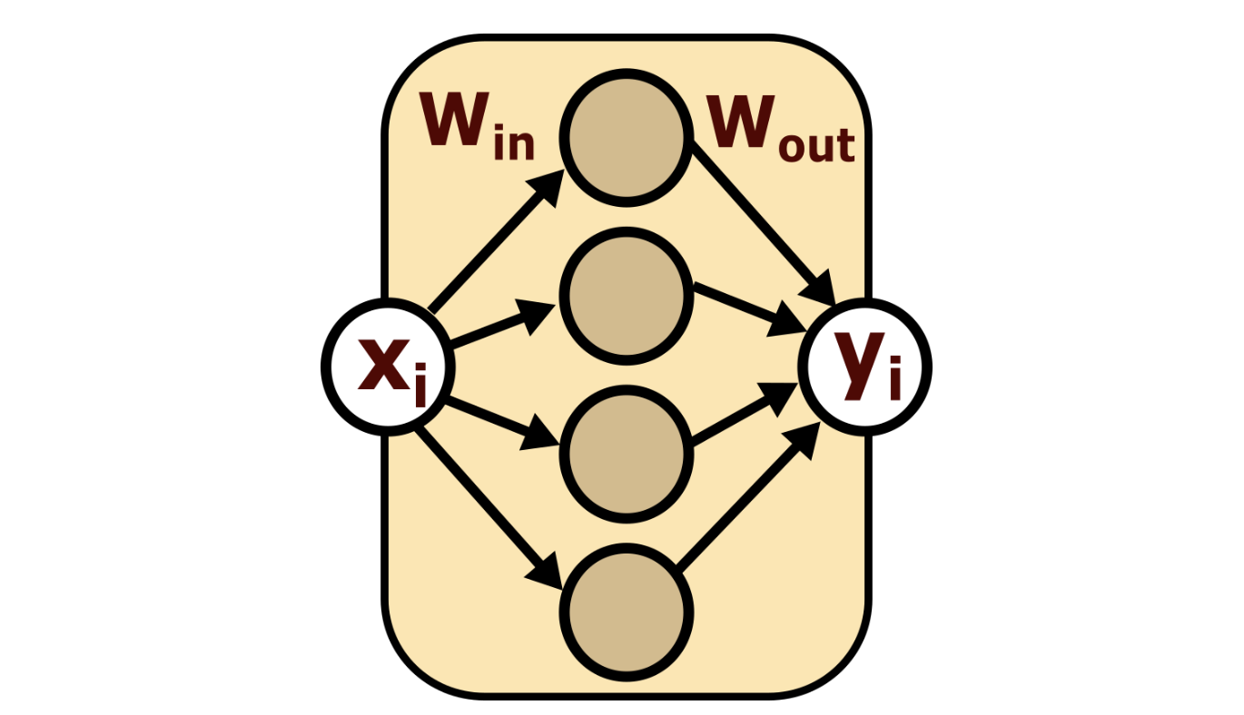
Based on "Transformer feed-forward layers are key-value memories", and based on my intuitions about ReLU (used in the OPT models), I decided to prune the MLP layers in quite a simple way, where my importance function for how important a neuron is in a dataset is its positive activation frequency.

• Importance = $\text{frequency}(\text{neuron activation}>0)$
• Scoring function = $\frac{\text{importance}\left(\text{cripple dataset}\right)}{\text{importance}\left(\text{focus dataset}\right)+ϵ}$

Then the method used was:

• Calculate the importance of each MLP mid-layer neuron for both the specific and general datasets (i.e: the activation frequency for each neuron in each dataset).
• Calculate the scoring function: the ratio of importances (i.e: the ratio of activation frequencies between the two datasets)
• Delete some top fraction of neurons based on the scoring functions.
  • That is, set the input and output weights and biases, $W_{IN}$, $B_{OUT}$ and $B_{OUT}$ to 0.0 for that neuron).

This was mostly based on the assumption that is a neuron is used much more frequently for one task compared to some second task, then it is likely more important for the first task than for the second. Current testing seems to indicate that this works relatively well for identifying task-specific neurons to delete. 

I did not expect that this method would cleanly generalise to other activation functions, but it seems to have worked similarly well for GeLU in the Galactica models. Still, there might be more room to think about better importance functions. 

 

2.4.2. Attention Pruning

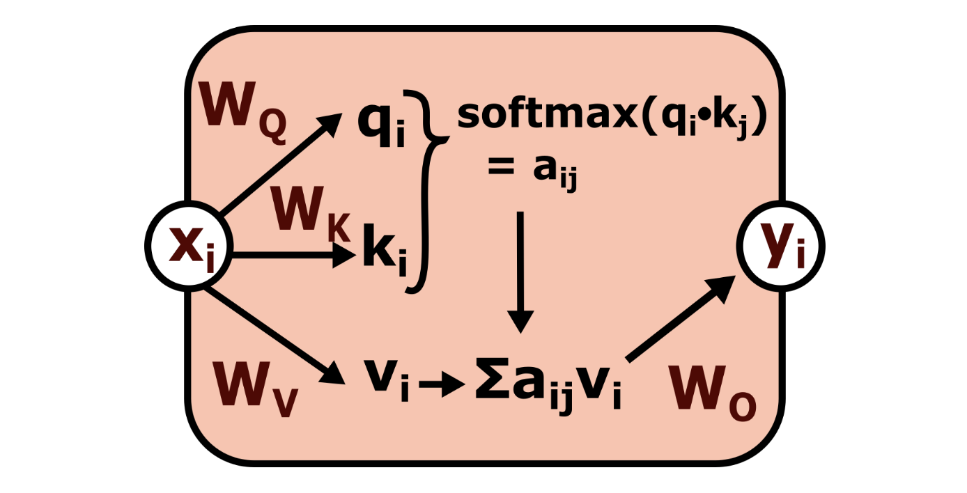
The output of the attention (ignoring how the $a_{ij}$ attention weights matrix is computed) is given by:

$$y_i=W_{OUT}\left(\sum _j{a}_{ij}(W_V\cdot x_j+B_V)\right)+B_{OUT}$$

We can write this diagrammatically, choosing to label the ${\sum }_j{a}_{ij}\cdot v_j$ as 'pre-out':

$$\left(x_i\right)\stackrel{W_V\left(x_i\right)+B_V}{\to }\left(v_i\right)\stackrel{a_{ij}}{\to }\left({\text{pre-out}}_i\right)\stackrel{W_{OUT}\left({\text{pre-out}}_i\right)+B_{OUT}}{\to }\left(y_i\right)$$

I mostly ignored how the ($W_Q{W}_K$) circuit works, and only look at the effect this has on pre out in the ($W_{OUT}{W}_V$) circuit. This means I likely lose out on being able to detect induction heads and similar, and for now I will just call that machinery "general" and leave that for future work.

I collect the activations of neurons in this "pre-out" layer. This was because I did not want do directly interfere with any of the dimensions of the residual stream, and only interfere with the adjustments made by the computational components (the attention and ff layers).

Since there is no activation function on the pre-out layer (other than the linear scaling induced by the attention weights), I need some other way of choosing the distributions that are most important. I tried analysing the distributions, and choosing which attention heads "contribute the most information", but I don't have a strong statistical background, so my methods were probably not very principled. My hope was to find some way of how much information a neuron contributes in two different datasets.

I tried to choose a few importance functions. I looked mainly at the activations at the "pre-out" state, and the main possibilities that I tried per neuron were:

• ${\text{importance}}_{std}$ = $\text{StandardDeviation}\left(\text{neuron activation}\right)$ 
• ${\text{importance}}_{abs}$ = $\text{Mean}\left(|\text{neuron activation}|\right)$
• ${\text{importance}}_{sqrt}$ = $\text{Mean}\left(\sqrt{|\text{neuron activations}|}\right)$

For motivations to the scoring functions I chose, see Appendix A: 

Note: that the standard deviation is calculated about the mean of each respective distribution. It might make more sense to have standard deviation about the mean of the base distribution instead.

The scoring function was then just the ratio of importances again:

• scoring function = $\frac{\text{importance}\left(\text{cripple dataset}\right)}{\text{importance}\left(\text{focus dataset}\right)+ϵ}$

For each neuron in what I will call the “pre-out” layer of an attention head (in the diagram above, represented as (${\sum }_i{a}_{ij}{v}_i$), calculate importance and scoring function for the tasks. The method was:

• Calculate the importance functions for all the activations of the neurons in the pre-out layers in a head for two different datasets.
• Compute the scoring function from the importances.
• Choose some top fraction of attention pre-out neurons
• Optional: Alter the biases to match the mean activation of these pre-out neurons.
  • That is, set $B_{OUT}^{\prime }=B_{OUT}+\text{Mean}\left(\text{pre-out}\right)$
• Delete these pre-out neurons.
  • That is, set the input and output weights and biases, $W_V$, $B_V$ and $W_{OUT}$ to 0.0).

 

Pruning Attention with SVD

One issue I suspected, was that I didn't think there was an "inductive bias" to move the activations to be along the basis of the neuron activations. To try to solve this, I used Singular Value Decomposition to change the weights of the attention MLPs to possibly be more separable (which is possible because there is no activation function).

The procedure I followed to SVD the attention matrices was as such:

• Get the $W_V$ and $W_{OUT}$ weights, and the $B_V$ biases for an attention head
• Store the $W_{OUT}\left(B_V\right)$ transformed biases
• Do singular value decomposition on $\left(W_{OUT}{W}_V\right)=U\cdot S\cdot V^T$ 
• Remove the rows and columns of zero rank (i.e: the ones that didn't exist before SVD)
• Set $W_V^{\prime }=\sqrt{S}\cdot V^T$ and $W_{OUT}^{\prime }=U\cdot \sqrt{S}$
• Calculate the inverse matrix: $(W_{OUT}^{\prime }{)}^{-1}$
• Compute the new bias, $B_V^{\prime }=(W_{OUT}^{\prime }{)}^{-1}\cdot W_{OUT}\cdot B_V$

So the new diagram looks essentially the same with the new matrices for each head, (but hopefully with the pre-out neurons better aligned for separability):

$$\left(x_i\right)\stackrel{W_V^{\prime }\left(x_i\right)+B_V^{\prime }}{\to }\left(v_i\right)\stackrel{a_{ij}}{\to }\left({\text{pre-out}}_i\right)\stackrel{W_{OUT}^{\prime }\left({\text{pre-out}}_i\right)+B_{OUT}}{\to }\left(y_i\right)$$

This SVD-ization method seems to work fine, and doesn't have a noticeable impact on normal loss before pruning (difference in loss seems to be about 0.01% on FP16), but I haven't done too much testing.

One thing to notice: Since the attention weight $a_{ij}$ is normalised by the softmax (so that ${\sum }_i{a}_{ij}=1$), we can instead just set the biases to be $B_V^{\prime }=0$ and $B_{OUT}^{\prime }=B_{OUT}+W_{OUT}{B}_V$, and still always get the same result (at least, before pruning).

 

Pruning Attention Heads

It also generally seemed that looking at SVD of the neurons, one can usually find that the attention heads mostly seemed quite related to each other (seen in "The Singular Value Decompositions of Transformer Weight Matrices are Highly Interpretable [AF · GW]", and "Branch Specialization"). So, trying to combine this per-neuron scoring information to per-head, we can use one of the following aggregation functions:

• $\text{mean}\left(\text{importance}\right(\text{neuron activations}\left)\right)$ for each neuron in a head
• $\text{median}\left(\text{importance}\right(\text{neuron activations}\left)\right)$ for each neuron in a head

Then one can compute the ratio to get a score for each head, and prune some top fraction of heads, optionally offsetting by mean activations.

 

2.4.3. Random Removal

Instead of the above methods, I also attempt to remove the same components, but instead of using statistical methods to choose which neurons and heads to delete, I instead choose randomly. This gives a baseline to compare the above procedures against.

 

2.4.4. Summary of Pruning Options

This was a lot of options, so I will summarise the different possibilities I tried testing:

Feed Forward Pruning:

• Importance Function:
  • Activation Frequency
• What level to prune on:
  • MLP middle layers

Attention Pruning:

• Choice of Importance Function:
  • StandardDeviation (std)
  • MeanAbs (abs)
  • MeanSqrt (sqrt)
• What level to prune the attention on?
  • Prune pre-out neurons
  • Prune whole attention heads
• $B_{OUT}$ bias offset: 
  • No offset
  • Offset by mean pre-out activations
• SVD the attention matrices $W_{OUT}$ and $W_V$?
  • Yes
  • No

If you are knowledgable about LLMs, then I recommend you try guessing what combination works best for separating out different capabilities, based on your intuitions about how LLMs work.

 

3. Results

3.1. Choosing the Best Pruning Method

You can view the data for this section on this weights and biases project (1)

In order to prune the models, we need to have a good understanding of how well the pruning methods above work, and how to choose how much we want to prune the Feed Forward layers and the Attention Layers. 

3.1.1 Pruning Galactica 1.3b

We start by looking at pruning Meta's Galactica-1.3B model.

The pruning was done in 20 steps, with each step either:

• pruning 5% of feed forward neurons, or
• pruning 5% of attention (heads or neurons) in various configurations.

The areas at each step of pruning we get at the end for each model, for Top1, Top10, Top10 Skip50, and Top1 Skip50 looks like this (respectively):

We also look at some pruning trajectories with Top10 and Top10 Skip50 performance accuracy:

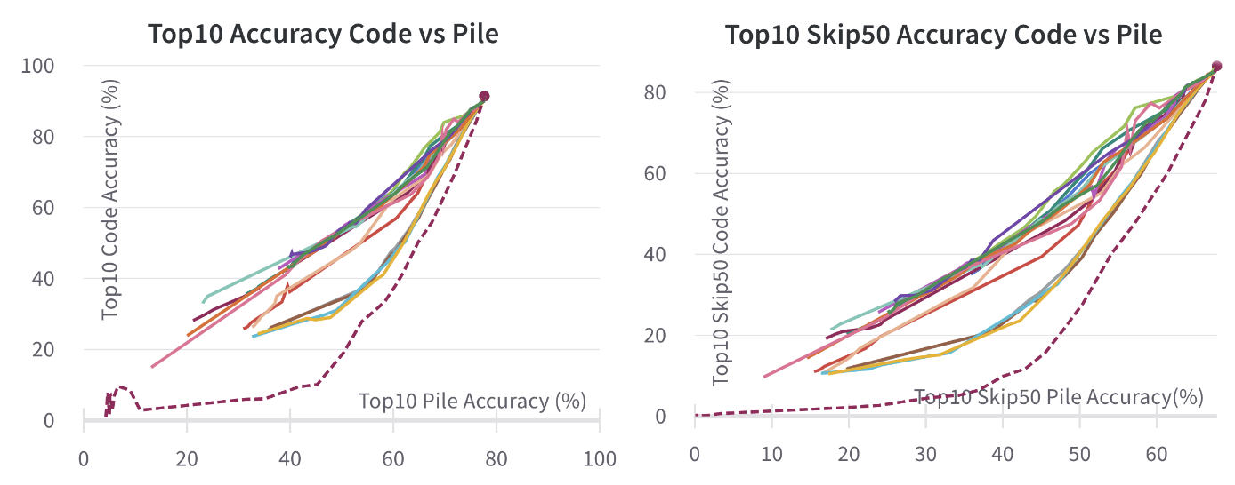
 We see that there are 4 main "groups" of outputs, in order from "best" to "worst": 

• ff: Feed Forward Pruning
• attn abs & sqrt: Pruning Individual Attention Pre-out neurons with SQRT or ABS
• attn std: Pruning Individual Attention Pre-out neurons with STDEV
• attn h: Pruning Attention Heads (using both mean and median metrics)

The singular value decomposition seems to have had relatively little effect (but possibly a very small negative effect) on how differential the performance loss was. Not shown in the graph, but I also tried offsetting the attention by the mean activations, and the performance was basically the same as the "attn h" category.

So based on this, we can somewhat conclude that:

• Pruning Feed Forward with counting works pretty well
• Pruning Attention is more difficult, doesn't work as well as Feed Forward pruning, and some methods are better than others, but it still somewhat works.

If we go back to our summary of attention pruning options. My interpretation of the results, is that we get:

• Choice of Importance Function:
  • StandardDeviation (std) - Moderately Bad
  • MeanAbs (abs) - Good
  • MeanSqrt (sqrt) - Good
• $B_{OUT}$ bias offset:
  • No offset - Good
  • Offset by mean pre-out activations - Large Bad Effect
• SVD the attention matrices $W_{OUT}$ and $W_V$? - Little Effect 
  • Yes - Good (but slightly worse than not?)
  • No - Good
• What level to prune the attention on?
  • Prune pre-out neurons - Good
  • Prune whole attention heads - Large Bad Effect

These results were surprising to me. I expected no SVD to be much worse than with SVD, but it seemed to have little effect (or possibly a slight negative effect?). 

For the most part, it seems like choosing the wrong neurons can lead to pruning being almost as bad as random, compared to the ideal results (of the ones I have tested). It seems like choosing better metrics might have a positive impact.

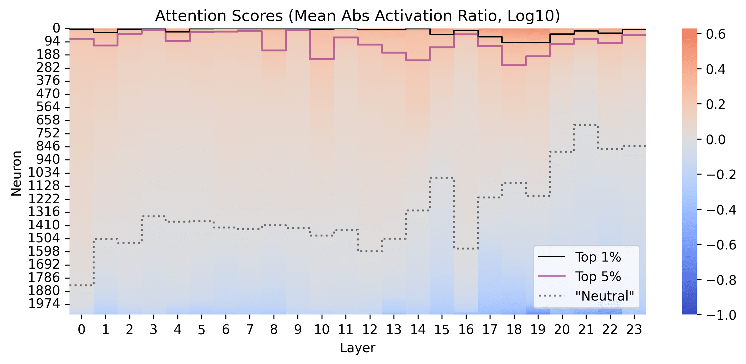
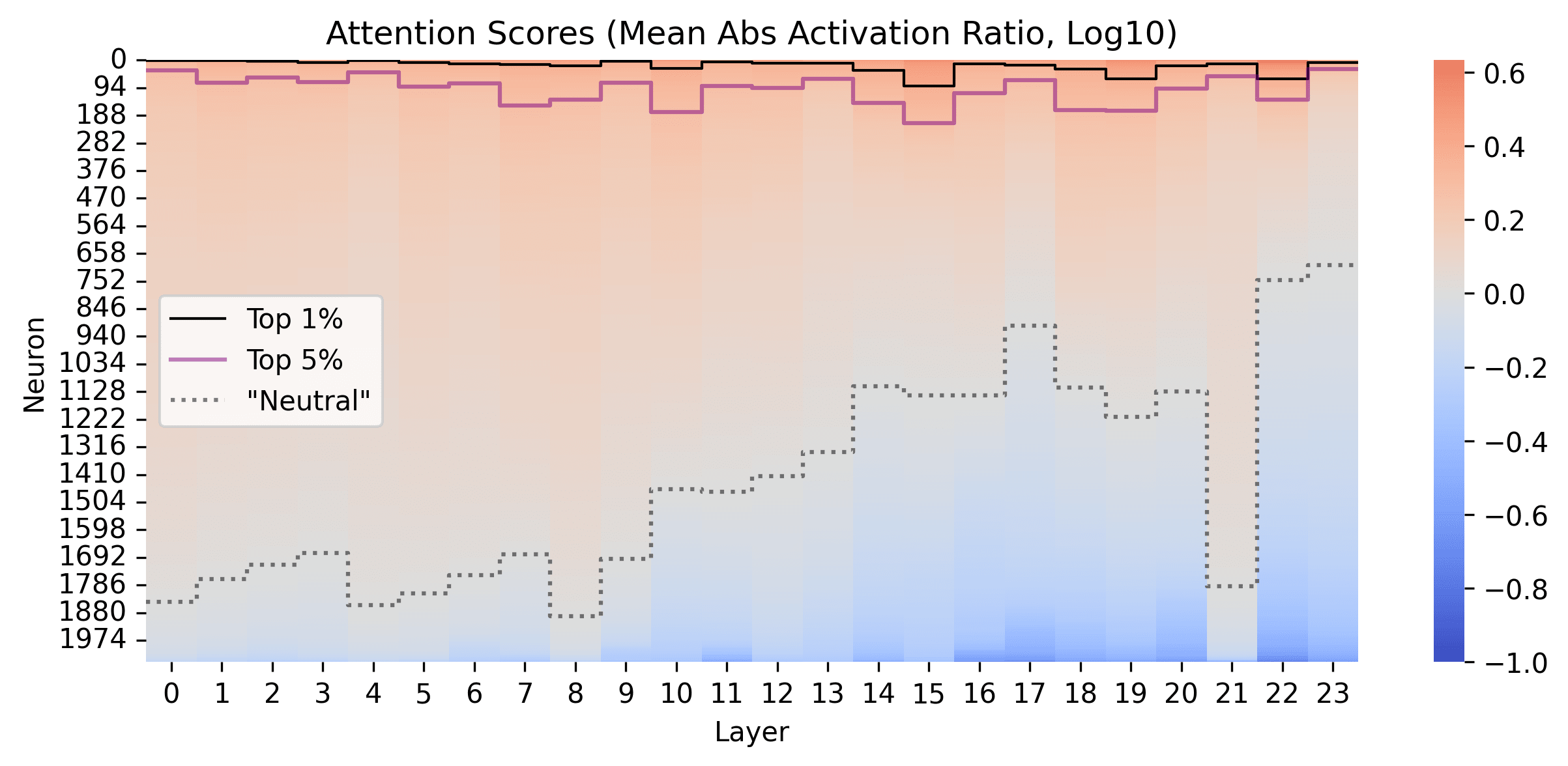
We also look at which neruons are being pruned in the Feed Forward and the Attention layers, by looking at how the scoring function evaluates the different neurons (log10)

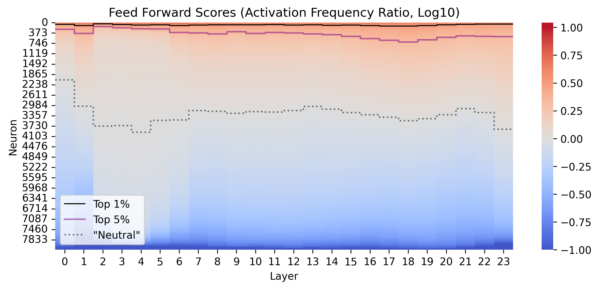
In the Feed Forward layers for Galactica 1.3B (post GeLU), it seems like mostly random whether a neurons activates more or less for the Feed Forward layers in Galactica, but there some small number of neurons that seem to activate more than 10x more in the code than in the pile, and some others that appear to activate more than 10x less.

We generally see quite smooth distributions, and that the early layers have a smaller proportion of neurons activating more for FF, and a more equal number activating more or less in later layers. Apart from the first layers, there doesn't seem to be much differentiation between layers

In the Attention heads, it seems that Code activates most neurons more than in the Pile. This might indicate that code is particularly sensitive to things that have been written before the most recent token. It seems here that there is a much larger difference between layers, possibly random variation dependant on some small number of heads. Early attention layers seem to be more general, and later attention layers seem to be more task-specific.

 

3.1.2. Pruning OPT 1.3b

Next, I present some pruning I did with Meta's OPT 1.3b. The 5 lines on the graphs are:

• opt 1.3b ff: Pruning 4% of the MLP each time step.
• slow opt 1.3b ff: Pruning 0.5% of the MLP each time step.
• opt 1.3b both (1): Pruning 4% FF and 1 attention head each time step.
• opt 1.3b both (2): Pruning 4% FF and 2 attention heads each time step.
• opt 1.3b attn: Pruning 7 attention heads each time step.

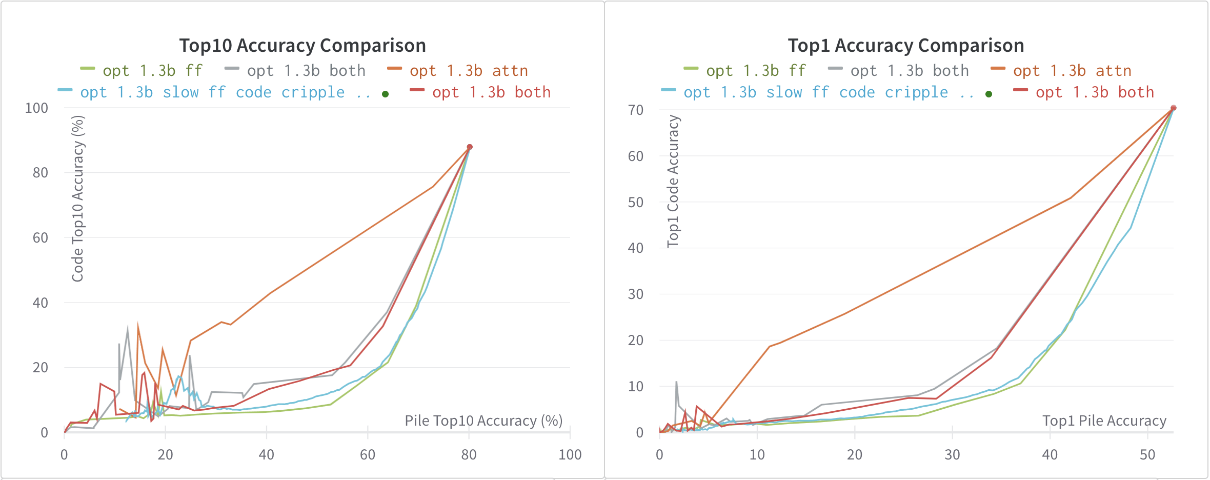
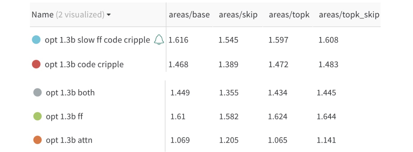
We first notice that for the most part, $\text{Attn}<\text{Both}<\text{FF}$:

• Pruning only the attention heads is unsuccessful.
• Pruning only Feed Forward layers is quite successful
• Pruning using both is mostly not as good as just pruning Feed Forward

We also look more closely on the Slow FF Pruning (small steps) and Fast FF pruning (large steps). We see that:

• Slow FF has a much smoother curve (since there are more data steps) than Fast FF
• Slow FF initially has better differential performance
• Fast FF pruning begins to have a worse differential performance 

I don't fully understand this. One hypothesis I have is:

• There are some late-layer neurons that mostly depend on early-layer computations.
• The early-layer neurons get deleted in an earlier time step
• The late-layer neuron no longer activates as differentially towards "code" vs. "pile", and now is more difficult to identify and prune, but still provides some value to the prediction.

We see in some parts where pruning both performs slightly better, but it is still non-obvious what the best method to do this is. In future research, if one is looking at pruning all the way, it might make sense to prune only FF, then later prune FF + ATTN.

In practice, what we likely care about is the initial performance differential, so in most cases, I would guess that it would be best to look at the slow pruning in detail. For this report, however, I will stick to fast pruning, because it is faster.

 

I also look at which neruons are being pruned in the Feed Forward and the Attention layers, by looking at how the scoring function evaluates the different neurons (log10)

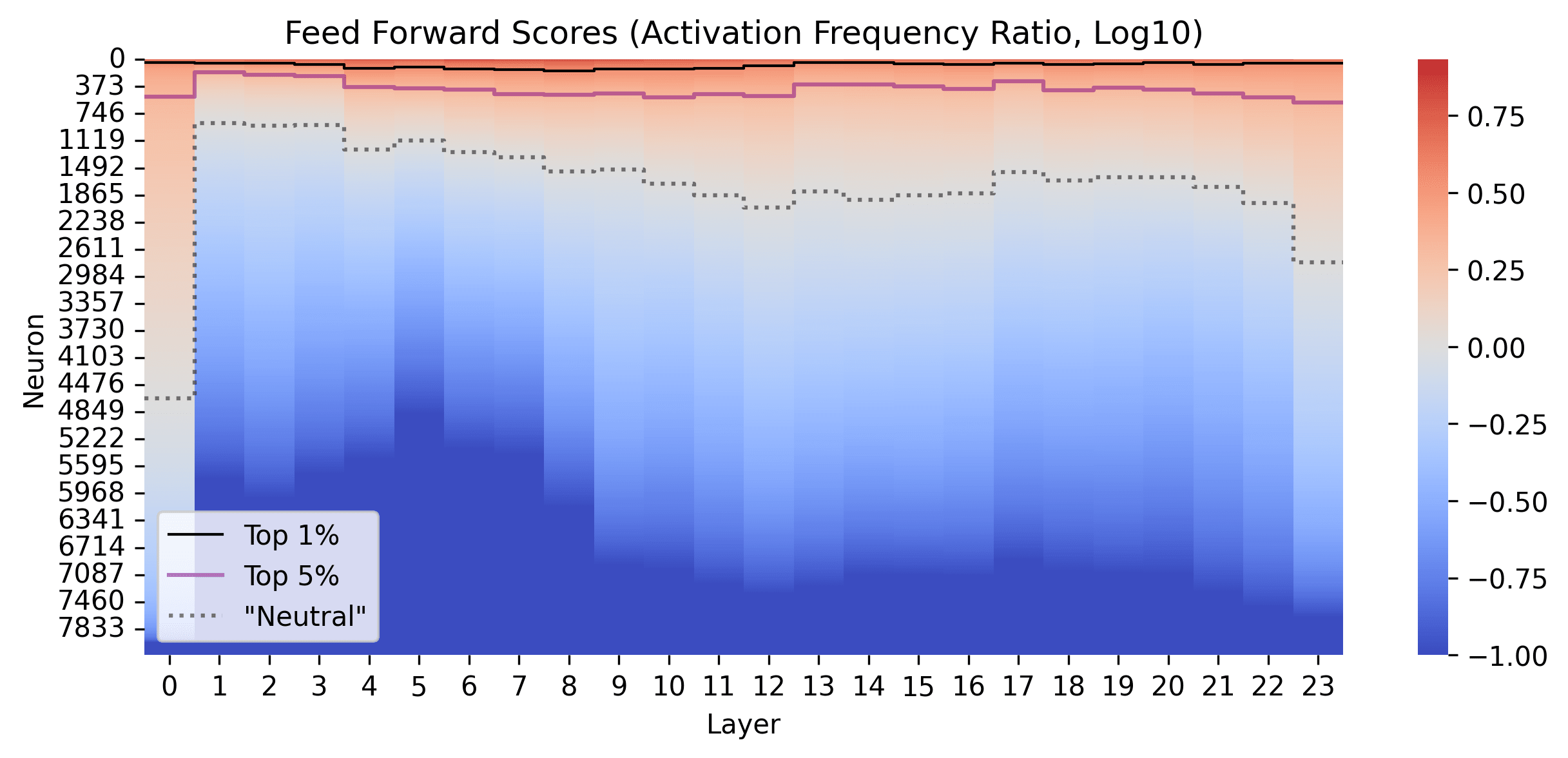
We see that in the Feed Forward layers in OPT-1.3b, the distribution is much sharper than in Galactica, and that a few neurons seem particularly specialised to Code compared to the pile.

I think this sharper distribution is likely due to the fact that OPT uses biases to down-weight neuron activations, while Galactica does not (but I guess could also be related to ReLU vs GeLU). I think this is supported by the fact that in most layers, over 80% of the biases are negative (though does not explain all the layers, since layer 2 seems to have mostly positive biases?)

In contrast, in the Attention layers, we don't seem to quite see the same separation, at least using the metric I have used, and see a pattern somewhat similar as in Galactica again: the early attention layers seem to be more general, and later attention layers seem to be more task-specific.

 

3.1.3 Bi-Directional Pruning - FF Only

We can try to compare the effects of pruning Feed Forward layers for both code cripple and code focus.

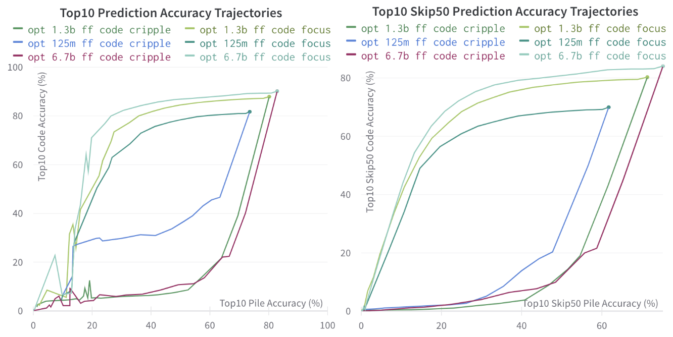
For larger models, the pruning trajectories look somewhat symmetrical. For small models (OPT-125M), we see that the Skip50 and non-skip accuracy trajectories do not line up. The Skip50 trajectory remains quite symmetrical, but for the normal non-skip Top10 accuracy, there is a substantial difference in OPT-125m:

• When pruning code cripple, it seems to get stuck at a level, where it has internalised and mixed representations of code and non-code text, and it is difficult to delete the code related logic.
• When pruning code focus, it seems more tractible for a longer time to remove english capabilities un related to code.

One thing we do notice, is that it seems generally that even in larger models, the code focus approach seems to hit somewhat of a wall. I suspect this might be because of things like "code contains lots of comments which requires good general english knowledge" and similar, but I am not sure.

 

3.1.3 Bi-Directional Pruning - ATTN Only

We now try to do the same looking at attentions only. I also add a comparison where I do random pruning on the MLP layers:

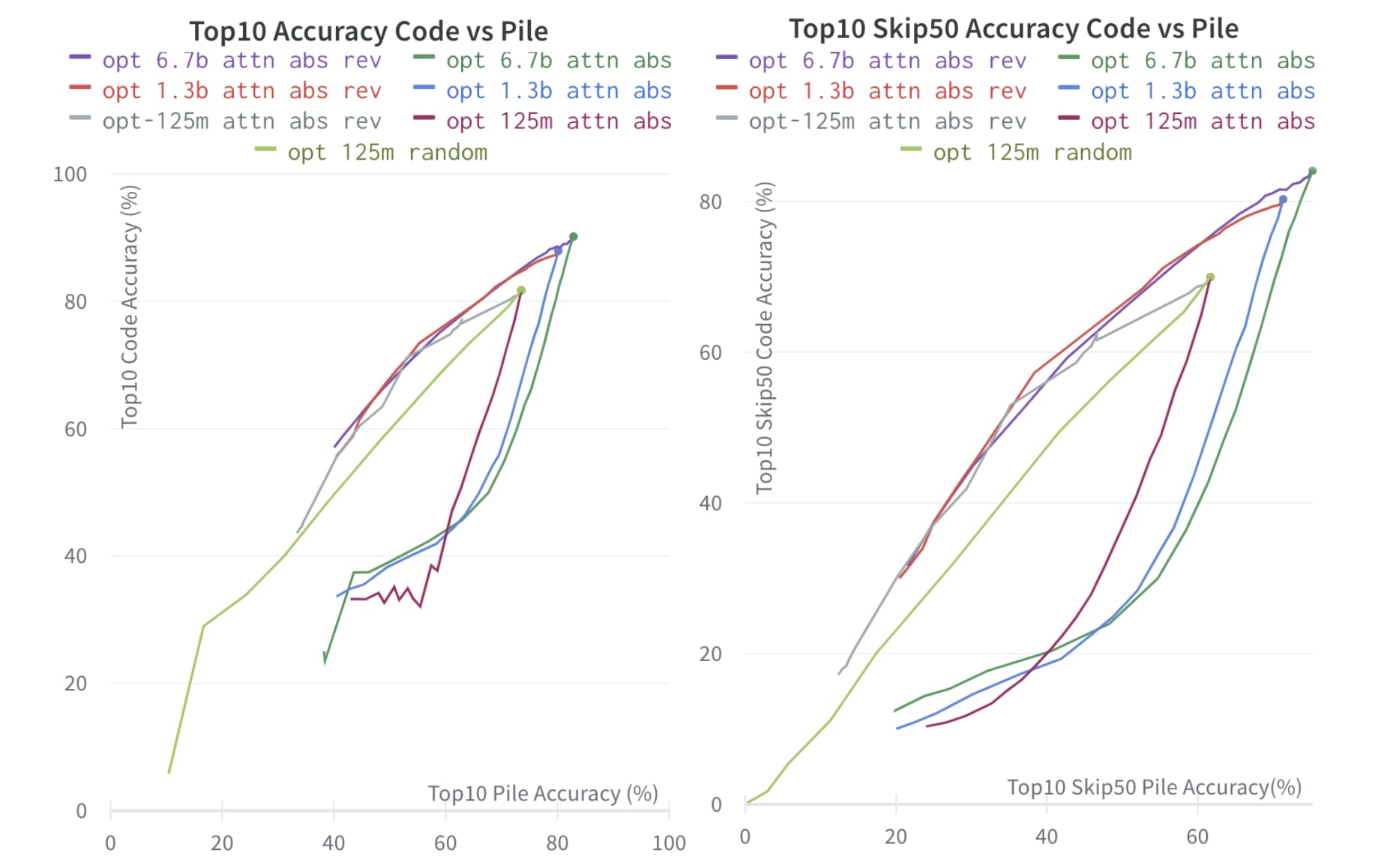
We see here that the pruning attention pre-out neurons work much better for code-cripple than for code-focus in all sizes of models. I don't have a complete understanding as to why this is happening. I vaguely suspect that the attention heads might mostly be providing general information, and that this is refined in specific scenarios. Alternatively, it might be that the metrics I am using don't work well bidirectionally. I think I will need to run more dataset comparisons to fully understand.

 

3.2. Pile vs. Code Separability in Meta's Models

You can view the data for this section on this weights and biases project (2)

We see that the models are moderately separable for Pile and Code for all the different sizes of OPT and Galactica models that I tested. I summarise the results with the following graph:

The main methods I tried were:

• "ff" pruning: Only pruning feed forward layer neurons
• "both" pruning: Pruning 5% FF and 2% ATTN pruning at each step

We look at the Pruning Trajectories:

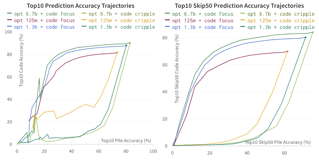
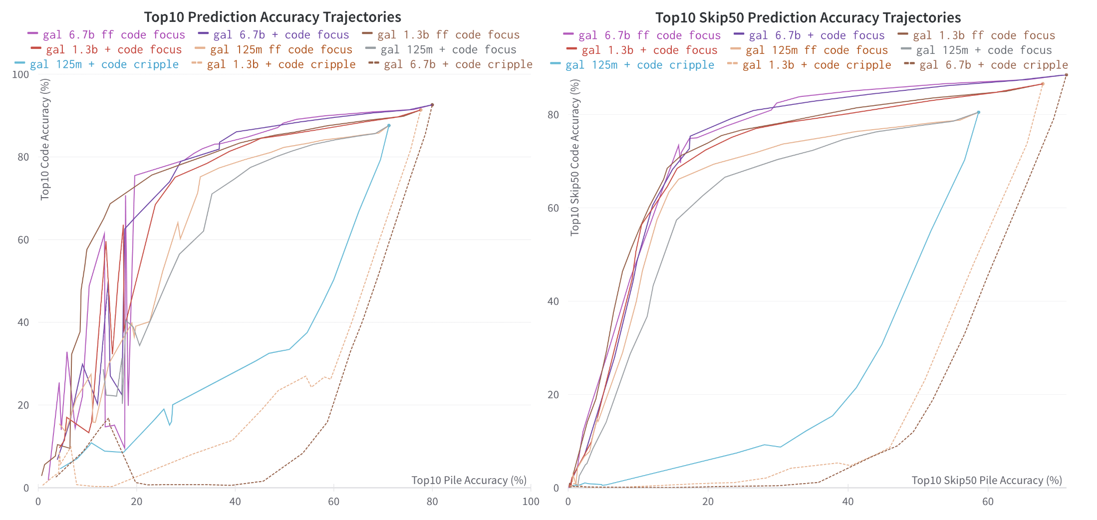
From the data (not all shown here), it seems mostly that for the OPT models:

• For code cripple, "both" pruning worked best
• For code focus, "ff" and "both" pruning were about equal

For the Galactica models:

• For code cripple, "both" pruning worked best
• For code focus, "ff" pruning worked best (but the difference is small for the larger models)

There are some further optimisation to be done with tuning how pruning occurs at each time step, but we can still get a rough picture of how well the pruning separates out the capabilities.

We look at the pruning areas for each:

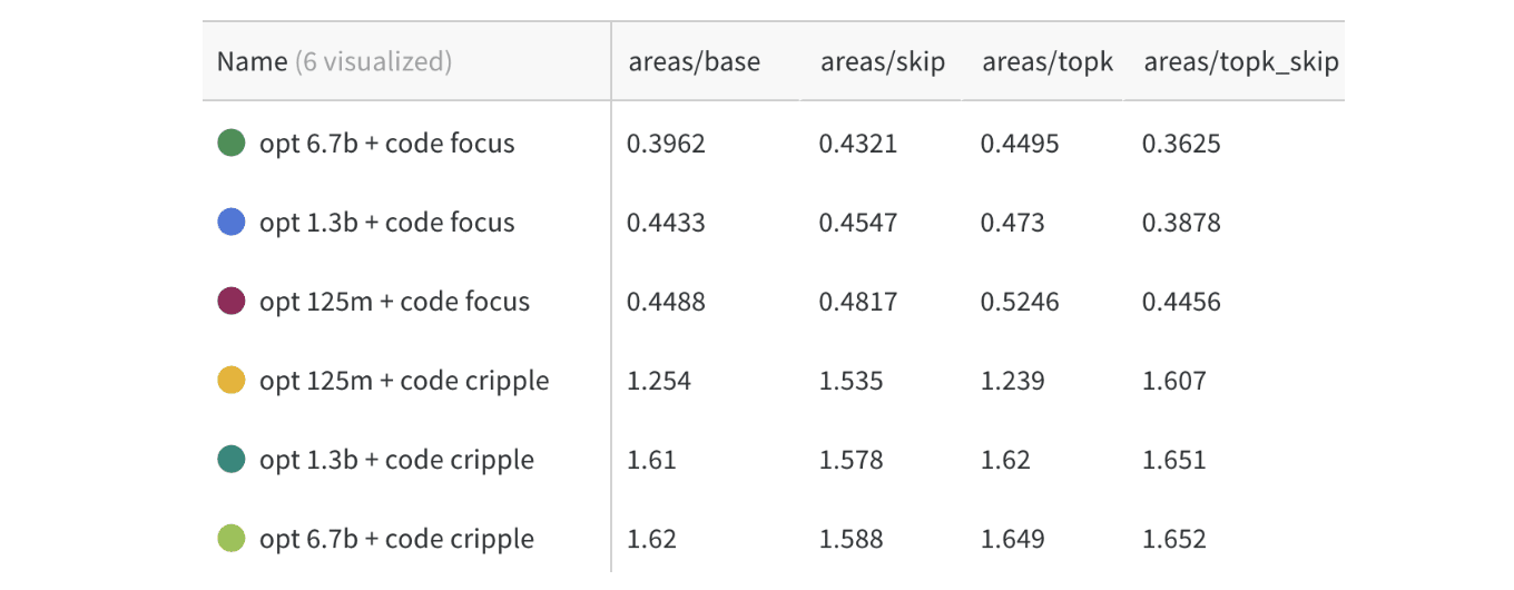
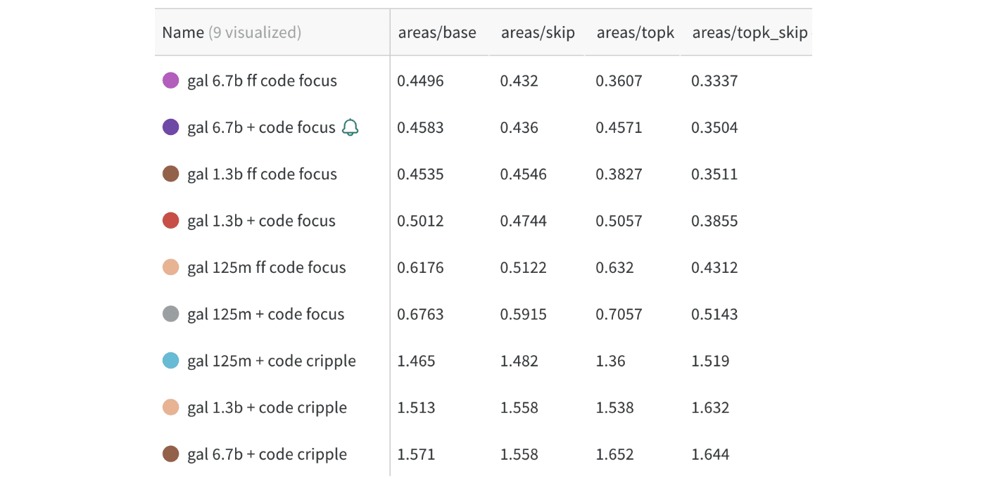
We see, compared the base area of 1.0, the areas are typically 0.3-0.7 for code focus, and 1.4-1.7 for pile focus, showing that we are roughly able to either remove or exclusively keep coding ability somewhat well.

One interesting result, predicted here [LW · GW], is that the larger models did seem slightly more separable/modular, but only to a small extent. I have not yet thoroughly tested the largest models (e.g: OPT-175B), but I expect that the result is roughly along the lines of "slightly more modular, but not by much" by these metrics.

Another interesting thing to note, is that the 125 million parameter models seem to hit a roadblock when looking at Top10 accuracy, at a level of about 30%, while in larger models, there does not seem to be such a roadblock. I suspect that there might be some task that is useful for both pile and code that gets separated out between the two in this situation, but I am not sure to the nature. (maybe for example, "code comments" begins to have it's own dedicated circuits?) 

 

3.3. Code vs. Python Separability in Meta's Models

You can view the data for these section on this weights and biases project (3)

We not look at a more difficult task: Separating out python capability from general coding ability. This is obviously a much more difficult task than the previous code vs. pile separability task, and we can see this from the charts below:

We can also look more in depth at the separability pruning trajectories:

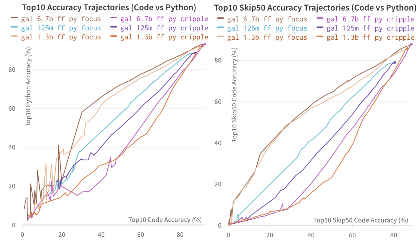
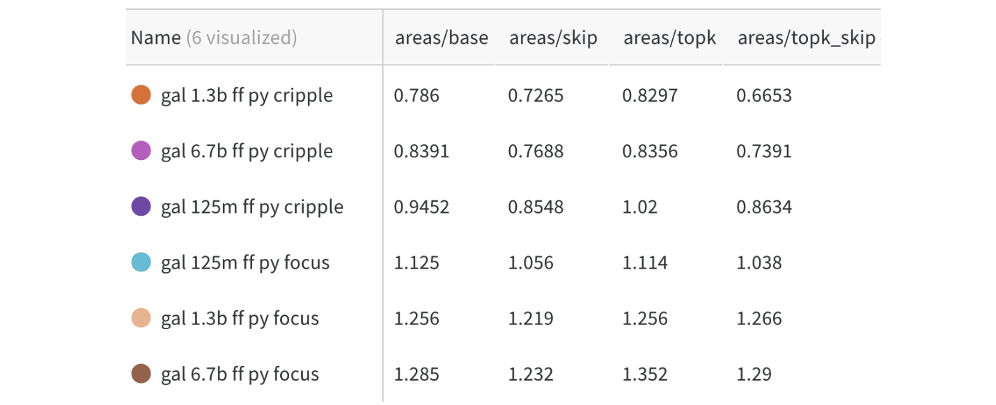
Unsurprisingly, it is difficult to separate out the parts of the model responsible for coding, and the parts of the model responsible for coding in python. We see that areas are stuck in the range of 0.7-1.3. 

We do, however, see that with the small models, the separability is really quite difficult, the pruning seems almost identical to random, and with the larger models, it seems to get easier to separate out the different knowledge required for each, perhaps showing an increase in modularity. However, more research is required.

 

3.4 Civil Comments

You can view the data for these section on this weights and biases project (4)

In order to compare my work with recent work, I quickly attempted to compare with the method described in "Editing Models with Task Arithmetic". Here, they fine-tuned a model for predicting text, and evaluated what proportion of comments generated (out of 1000) were toxic, and their mean toxicity. Here are their results for GPT-2 Large (774M parameters):

Method	% Toxic	Mean Toxicity	WikiText-103 Perplexity
Base Model	4.8	0.06	16.4
Negative Vector	0.8	0.01	16.9

While not exactly comparable, I attempted to try doing two pruning steps (total of 2% FF, 1% ATTN pruned) with OPT-1.3B, and could quickly replicate similar results:

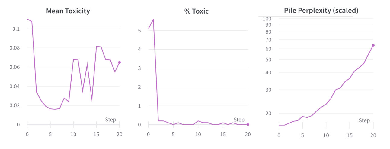
OPT 1.3B	% Toxic	Mean Toxicity	Pile Perplexity	Perplexity (rescaled)
Base	5.1	0.11	43.4	16.40
Pruned	0.2	0.03	45.3	16.87

We see that the decrease in toxicity as well as performance is approximately comparable, (better on one metric, but worse on the other), but this might also be due to using a larger model (1.3B vs 774B), which they had shown is easier to tune in this way.

One limitation however, is that while the percentage of comments generated that were above the threshold for toxic (0.8) dropped and stayed low, the toxicity score dropped and then rebounded with further pruning:

 

3.5. Other Observations

3.5.1 "Backup" Mechanisms

One somewhat annoying fact when trying to reason about transformers, is that there is a lot of what looks like redundant/”backup” mechanisms from training process. What this means, is that you can have strange behaviours. For example, one could have a Piece 1 and Piece 2, both doing the same task, and get behaviour like:

• Delete Piece 1 and no drop in performance because of Piece 2 still working
• Delete Piece 1 with a drop in performance, then after further deletions, Piece 2 has the right conditions to activate, and the performance goes back up

 

3.5.2 Threshold Spikes

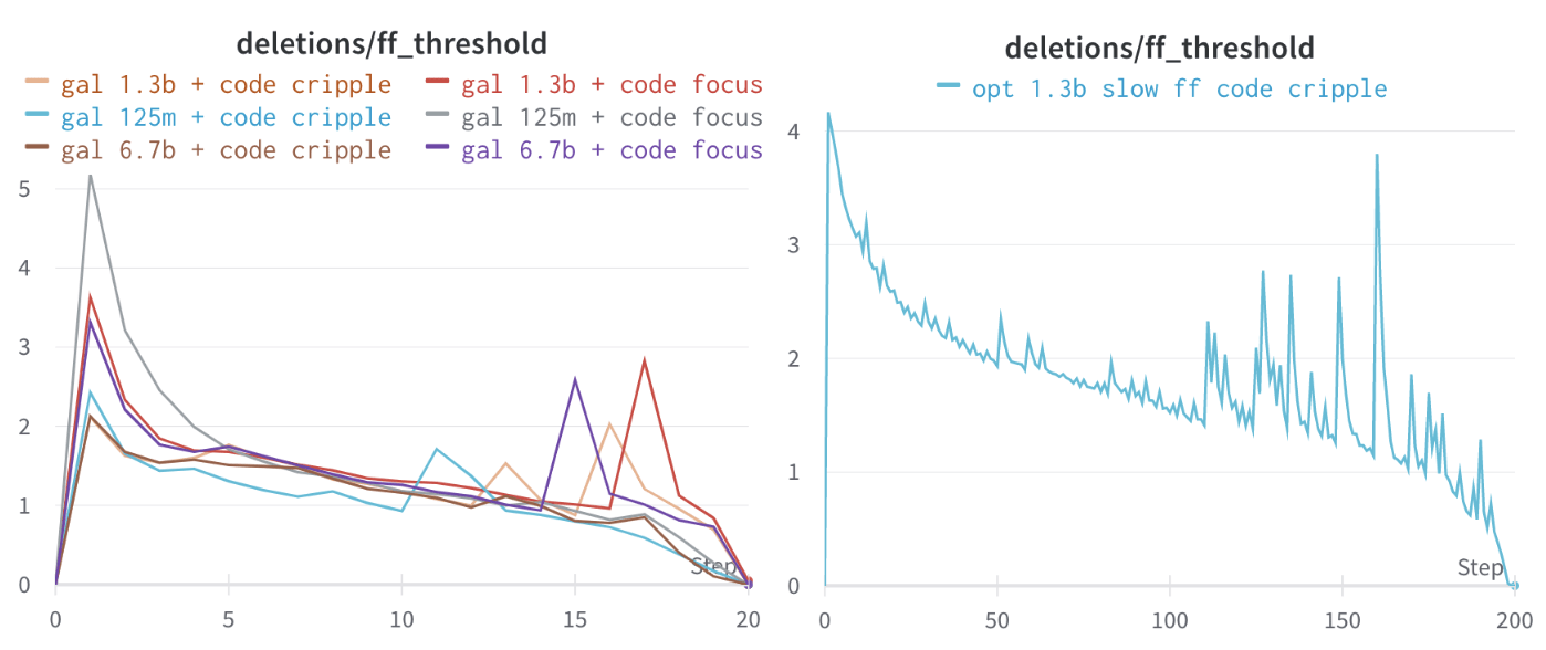
After deleting some neurons, there is often a decrease in performance for a few steps, until there is a significant jump in performance again. Though it is true my sample sizes are not that large and there may be noise, in this case it seems clear that that is not the issue.

Here is a graph of how the lower threshold of a 4% cut-off ratio looked like in different steps of the process. The step 0 is just a pre-test, and after, the cut-off is quite high, but slowly drops as we keep removing the most active neurons. At some point, however, the profile of neuron activity changes and there is a big difference in activation distribution.

One vague hypothesis is along the lines of Transformer feed-forward layers build predictions by promoting concepts in the vocabulary space, where the feed forward layers are responsible for the promotion and demotion of concepts. It might be that some “concept demotion” neurons get deleted, and so, the effect is that the general concept of coding is once again accessible.

In particular, in the MLPs, I have usually used the same % top relative frequency as a way of choosing which MLPs neurons to delete, and store the minimal threshold. This usually decreases, but can suddenly jump.

 

3.5.3 Late-Pruning Performance Jumps

One potentially strange phenomenon that occurs, is that after the $n$-th time pruning, performance increases instead of decreasing.

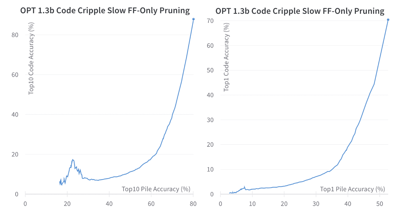
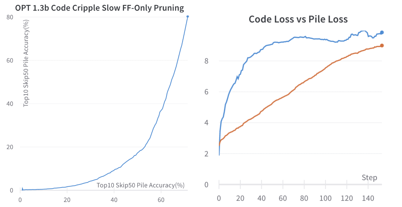
Some factors that might be causing this:

• There could be "code inhibition" neurons, such as in "Transformer feed-forward layers build predictions by promoting concepts in the vocabulary space", which get deleted and this improves performance.
• This seems to mostly only affect the 50 most common tokens, so some bias towards choosing the most common tokens might be helping after pruning a large amount of the model
• These metric only looks at a top-k cutoff, and there might be some other relevant token that no longer gets predicted

See further discussion in "further work".

 

3.6. Limitations

One important limitation, is that I have only been looking at next-token prediction. This is not actually a task that anyone cares about, but serves as a useful proxy for this early research. In particular, I look at a large range of prediction accuracies, but in the future, it would likely make more sense to look only at the losses that are "sufficiently close" to the original loss, since small changes in loss can lead to large differences in capabilities. This might mean that the results of this procedure are worse than shown above.

Another limitation, is that I only looked at total performance in the pile and code, instead of trying to look at a subset of the pile that does not contain any code. This might mean that the results here are better than shown above.

In addition, the measures of separability here are limited to the pruning techniques here on the models, rather than showing the true separability of the model, and these measure might not actually be that useful anyway.

 

4. Understanding What is Happening

4.1. Attention vs. MLP

My understanding of how transformers work, is that:

• The Attention heads collect relevant information
  • Key-Query circuit chooses where information comes from
  • Value-Output circuit chooses what insights to get from the information
• The Feed Forward layers do Key-Value concept promotion

Based on my findings, my current understanding is that the models are very Task-specific with the MLP layers, at least to a first-order approximation. The Attention heads seem to be more general, and seem to process information in a way that seems more general to both tasks.

Though I haven't tested any pruning on the Key-Query circuit, based on pruning attention heads vs pre-out neurons, I suspect (with no experimental basis) the $W_K{W}_Q$ circuit is very general, and (with more experimental basis) that the $W_{OUT}{W}_V$ is somewhat more task-specific.

Here is a rough diagram of my intuitions:

In addition, I think that the attention in earlier layers seem to be much more generally acting than attention in later layers. (for example, maybe something like "convert previous few tokens into the real word" in early layer vs "do task relevant thing" in later layers).

In small models, it looks to me like some of the attention + MLP combinations are combined, so that the attention head gives an approximation of the possible attention + MLP combinations. 

My vague explanation, is that:

• The model first learns to a first-order approximation things needed for all tasks, and since there are only a very small number of attention heads (and the possible number ways attention weights can be used is very limited), so they need to be useful for all tasks.
• The generally useful attention heads are combined into "circuits", that rely on the MLP layers to get the final information.
• The coding parts of the pile provide enough pressure to dedicate small amounts of computation in the model for them such as some MLP neurons, and to perhaps use some part of the attention heads, but not enough to dedicate whole attention heads to code that are not also useful to other tasks.

In very large models, it might be again the case that some of the attention heads would start to learn very task-specific features again, (particularly if it is past the return of having enough attention heads needed to do all the general things one could require) but I have not tested this.

To further investigate this hypothesis, I believe that examining the following points could be helpful:

• Clearer distinction: It would be interesting to see if the results demonstrate a more pronounced distinction between the roles of attention heads and MLP layers across a wide range of tasks, suggesting that attention heads are consistently more general while MLP layers are more specific.
• Consistent patterns across model sizes: Observing consistent patterns in the roles of attention heads and MLP layers across various model sizes could provide additional support for the hypothesis, as it would suggest that the observed roles are not artefacts of a particular model size or architecture.
• Fine-tuning results: Exploring the same hypothesis using fine-tuning instead of pruning might offer additional insights and help confirm whether the results align with my initial hypothesis.

However, there are alternative hypotheses that could be considered:

• Perhaps my pruning methods are insufficient to truly task-separate out the attention neurons.
• I haven't actually looked at the Key-Value attention heads
• Attention heads and MLP layers might be complementary, with both contributing to task-general and task-specific aspects, but in different ways, or at different stages of processing.
• The distinction between attention heads and MLP layers could be more nuanced, with some attention heads and MLP layers being task-specific while others are task-general.

I think further research is needed to explore the roles of attention heads and MLP layers in transformers across diverse tasks, model sizes, and methodologies such as fine-tuning.

Looking at more diverse tasks, consistent patterns across model sizes, and alternative methods (like fine-tuning) supporting or contradicting this hypothesis could provide stronger evidence either for or against this explanation.

Note that this hypothesis is particularly likely to be incorrect.

 

4.2 The Basis of Computation Might Be Neuron-Aligned

I was quite confused at first at why Singular Value Decomposition did not improve the performance of pruning the attention heads, and in fact seemed to slightly hinder pruning. However, I think I have some vague intuitions on what might be happening, which somewhat makes me suspect that neurons might actually already be in the correct basis in which to understand neural networks.

 

4.2.1 The "Curse of Dimensionality" means that most vectors are almost orthogonal

Another thing to consider, is the "curse of dimensionality". If one has a high-dimensional space (for example, 2048), and one chooses some random collection of vectors (eg: 50000), then one will find that most of these vectors are basically orthogonal to each other.

In particular, the distribution of cosine similarities between any two unit vectors vectors in an $n$-dimensional space is proportional to $(1-|x|{)}^{n-2}$, which has a sharp peak at 0. (for n=2048, over 87% will have cosine similarity less than 0.001, and over 99.995% of vectors have cosine similarity less than 0.005).

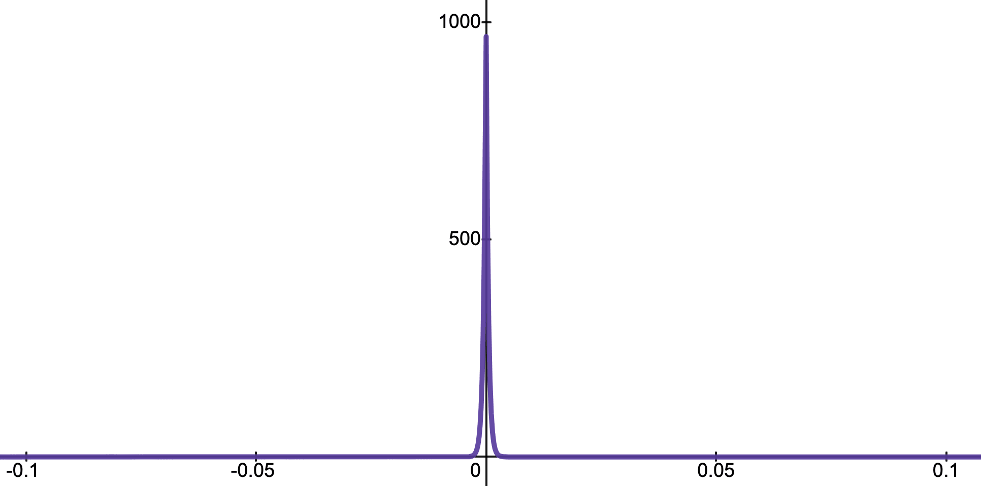
This means that if you have unit vectors, it is quite difficult to align them together, so SGD might have an inductive bias to use a basis of computation that is aligned with the directions of the neurons. Of course, the matrices of a neural network are not restricted to being unit length, and this does not strictly limit the neural network to using a basis that is neuron-aligned, but I think this would be an inductive bias.

In practice, we see that the magnitudes of the row vectors in the $W_V$ matrix are quite similar in magnitude to each other in within most layers except the first (usually within about a factor of two), so I suspect that the effect of the "curse of dimensionality" might be playing a significant role to align the basis of computations with the neurons in the self attention.

If one additionally adds L1 weight decay when training a model, I would expect that the neuron-aligned basis would have an overwhelming inductive bias (though my understanding is that in most models, when weight decay is used, the preferred type seems to be L2).

 

4.2.1 SVD can be disrupted by noise

An alternative explanation is that SVD is just not a useful tool in this scenario.

In linear algebra, if one matrix has two of the same eigenvalues, it is known as a repeated or degenerate eigenvalue. When this occurs, the eigenspace corresponding to that eigenvalue might have more than one linearly independent eigenvector, and any linear combination of these eigenvectors is also a valid eigenvector.

Analogously, in SVD, one can get degenerate singular values, and the orthogonal vectors corresponding to these values are not unique, and can be rotated. Alternatively, if one has two or more non-degenerate (but very close in value) singular values, and you add noise (such as one could get from SVD), then one could get a singular value vectors which are rotated, and which no longer corresponds to the "true" basis of SVD.

This might mean that the neurons are not the basis of computation, and that there is in fact a better basis of computation we could be looking at, but due to random noise, it is difficult to identify it. A different method could possibly work better.

 

In addition, there is recent work "Eliciting Latent Predictions from Transformers with the Tuned Lens", which seems to improve on the Logit Lens, but I have not yet tries to integrate this into my research yet.

  

Overall however, I this has updated me more towards thinking that computations are likely to be inclined to be aligned with that neuron, rather than some rotation between two or more neurons. 

 

4.3. Further Work

While the work here shows an initial promise for a way of thinking about modularity of Large Language Models, looking at Separability of Capabilities, it still requires a moderate amount of work to be used in full. There are a lot of things I still want to understand (and I may or may not get around to), but will likely take more time, so I am publishing early. In particular, a non-exhaustive list is:

1. Attempt to do the same experiments, but with fine-tuning instead of pruning.
   1. This can give a baseline on how separable the two tasks are in the first place.
2. Investigate model performance metrics that are more meaningful.
   1. So far, the only task being looked at is next-token prediction. It might make sense to look at a more interesting task, such as the various kinds of knowledge tests.
   2. The "areas" seem like an OK metric for separability, but lack some important features, and probably doesn't focus on the right things.
3. Better separate out task datasets.
   1. So far, I have used the whole "pile" and "code" sets, without the capability that is trying to be removed being removed from activations or evaluations. It might make sense to remove these beforehand to get a more accurate picture of the results.
   2. It might make sense to only collect activations for next token-predictions when they are accurate (but this method may also have pitfalls).
4. Attempt to understand small vs. large pruning steps better.
   1. It seems that smaller pruning steps can lead to better separability initially, but later in the pruning process, it can become much worse at separability.
5. Optimize pruning parameters.
   1. The current pruning methods use pre-defined top fractions of neurons and heads to prune. One could investigate ways that pruning more MLP first then ATTN later, or vice versa, could lead to better separability pruning.
6. Look in depth at what neurons exactly are being pruned at each step
   1. Compare which neurons are being pruned in the two different scenarios, and see if there is any overlap
7. Layer-by-layer pruning.
   1. It might be the case that there are instabilities to pruning neurons in all the layers at once, so it might be useful to prune layer-by-layer starting at the final layer. This could make it more likely that when there is pruning, that the whole circuits (not just some critical part) of the coding capabilities are removed.
8. Try to make pruning work on the entire "circuits", not just parts
   1. It seems likely that current pruning works mainly to sever some important part in the information chain, rather than prune the whole circuit. While this might be fine for some applications, I would prefer to have a better map of the neural networks from this if possible
   2. Preliminary testing seemed to show that inverting the neurons that were pruned for "code cripple" lead to basically zero performance, since the "general" parts of the network still remained.
9. Do a more in-depth analysis of exactly how much performance pruning each neuron causes
   1. One could prune 1-by-1 all of the neurons in a Galactica-125M. (~9216 attention pre-out neurons, and the ~36864 feed forward neurons), and evaluate the actual performance drop caused be each.
   2. This seems unlikely to work amazingly (due to backup circuit interactions), but could give some good insight if done well. With my current setup, this would take about 30 days, but one could run many instances on one GPU, and also use more GPUs, so seems doable.
   3. One could then try all sorts of metrics, and find the best metrics that seem to work for this model.
10. Better pruning for MLP Layers.
    1. Basic positive activation counting seems to work quite well, but it seems possible that there could be better methods.
11. Better Pruning for Attention Heads.
    1. Maybe there are better scoring functions for choosing which attention heads to prune?
       1. For example, compute standard deviation from a common mean for both datasets?
    2. In particular, there might be a few heads with multi-modal distributions, which makes it difficult to pin down "activation importance". 
12. Attempting to better integrate understanding in the $\left(W_Q{W}_K\right)$ attention circuit. How does one try to think about separability there? Are there heads which have two or more "modes" of activation?
13. Attempt to fully understand jumps in performance after some pruning steps:
    1. This might be because there are other parts that do a slight signal boost to the correct prediction, that gets drowned out by other signal boosts.
    2. The performance jump mostly happens on most common tokens. Maybe there is just a bias toward predicting the most common tokens?
    3. This might also be because the embedding and unembedding have a prior on bigram predictions to make net-token prediction accurate.
14. Attempt to fully understand slow vs. fast pruning:
    1. Pruning slowly is better at first, but worse later on. Why? What causes the metrics to be failing?
15. Better understand how to offset biases
    1. From my testing, offsetting by the mean activation didn't seem to work
    2. I am not sure if I should delete the original biases, or if I should combine them. Probably more testing is needed here, though I think that for large models, biases don't make that much of a difference.
    3. This might not matter that much if future models do not use bias terms

 

As a longer term research direction, my aim is to try to understand the difference between "tasks" and "goals", and attempt to understand what "longer-term goals" might look like in a Language Model. I think that attempting to make the neural networks more separable might be useful for this, but this looks like it might come for free with larger language models.

• While so far there is some understanding of how next-token prediction happens, and while this might be enough to explain what is happening in the model, I am interested in how these local next-token predictions lead to a long-term direction for outputs the model tends to make.
• While it might be the case that FF and Attention neurons might be the basis for these tasks, it seems likely that there are in-built biases in the embedding space that make some paths of text more likely than others.

 

5. Conclusion

We can conclude that, at least to some extent, we can call current language models somewhat modular (using the metric of "separability area percentage" between two capabilities). When looking at code vs general text, I could get up to about 65-75% separability with current techniques. Python vs code separability seems to vary more by model size, from being <10% separable in small models (125M), to 25-35% separable in larger models (6.7B). These techniques, combined with the work of "Emergent Modularity in Pre-Trained Transformers" show some early insight into how one can think about modularity of language models, but there is a huge amount of work to still be done to build a full understanding.

 

6. References

Bushnaq, Lucius et al. "Ten experiments in modularity, which we'd like you to run! [AF · GW]", The AI Alignment Forum, 16 Jun. 2022, https://www.alignmentforum.org/posts/99WtcMpsRqZcrocCd [? · GW].

Bushnaq, Lucius et al. "What Is The True Name of Modularity? [AF · GW]" The AI Alignment Forum, 1 Jul. 2022, www.alignmentforum.org/posts/TTTHwLpcewGjQHWzh [AF · GW].

Pfeiffer, Jonas, et al. "Modular Deep Learning." arXiv preprint arXiv:2302.11529 (2023).

Zhang, Zhengyan, et al. "Moefication: Transformer feed-forward layers are mixtures of experts." arXiv preprint arXiv:2110.01786 (2021).

Zhang, Zhengyan, et al. "Emergent Modularity in Pre-trained Transformers."

Michel, Paul, Omer Levy, and Graham Neubig. "Are sixteen heads really better than one?." Advances in neural information processing systems 32 (2019).

Burns, Collin, et al. "Discovering latent knowledge in language models without supervision." arXiv preprint arXiv:2212.03827 (2022).

Belrose, Nora, et al. "Eliciting Latent Predictions from Transformers with the Tuned Lens." arXiv preprint arXiv:2303.08112 (2023).

Zhang, Susan, et al. "Opt: Open pre-trained transformer language models." arXiv preprint arXiv:2205.01068 (2022).

Taylor, Ross, et al. "Galactica: A large language model for science." arXiv preprint arXiv:2211.09085 (2022).

Geva, Mor, et al. "Transformer feed-forward layers are key-value memories." arXiv preprint arXiv:2012.14913 (2020).

Millidge, Baren and Black, Sid. "The Singular Value Decompositions of Transformer Weight Matrices are Highly Interpretable [AF · GW]." The AI Alignment Forum, 28 Nov. 2022*,*
 www.alignmentforum.org/posts/mkbGjzxD8d8XqKHzA [AF · GW].

Voss, Chelsea, et al. "Branch specialization." Distill 6.4 (2021): e00024-008.

 

For the code used in these experiments, see: github.com/pesvut/separability

For the raw data, see weights and biases (sorry for the misspelling of separability): 

• 1: pile-code-attn
• 2: seperability-pile-code
• 3: seperability-code-python
• 4: civil-toxic

 

Appendix A: Choosing Scoring Functions for Attention Neuron Distributions

When trying to understand these activations,, one particular annoyance is that most of them are very non-Gaussian. Most activation distributions look mostly like a double exponential ($e^{-|x|}$) around zero, while some exceptions look more like Gaussians about some value, and others looks like somewhere in between both, and others look different again.

Idea 1: If a neuron activates a larger range of distributions for one task than for another task, then it is probably providing more information for that task. Does this mean, if the standard deviation is larger, then that means that it is more important? For example, see this diagram:

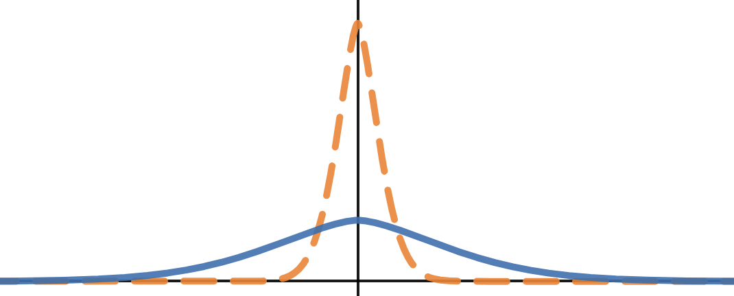
For this reason, I chose standard deviation about the mean ("std") as a scoring function. (though most of the distributions were not Gaussian, this is still the most common metric of variance). 

Note: that the standard deviation is calculated about the mean of each respective distribution. It might make more sense to have standard deviation about the mean of the base distribution instead.

Idea 2: Maybe what we care about is actually how much it activates as non-zero. For this, we can use scoring such as mean of absolute activations, or mean of square root of absolute activations as scoring functions. This seems likely to work well if we are setting the weights to zero.

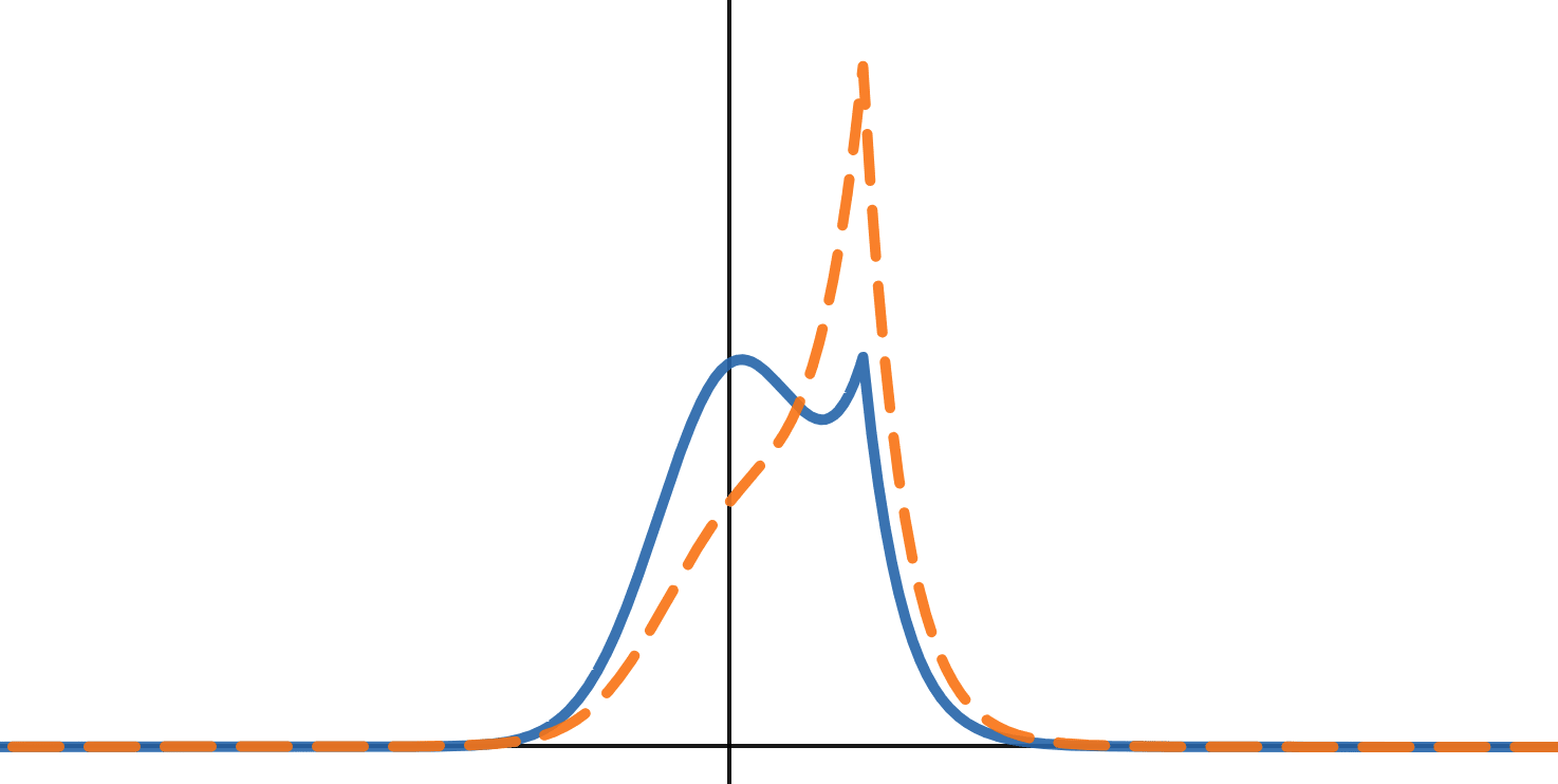
For this reason, I chose the metric of mean absolute activation from 0.0 ("abs") as a metric. However, this might mean that slight shifts in a Gaussian far away from the mean could have a big effect, so I also tried mean square root of absolute of value activation from 0.0 ("sqrt") as a metric.

In practice both of  "abs" and "sqrt" seem to work similarly well, and much better than "std", so I have mostly resigned to using this for now.

Some examples of distributions

Here are some interesting neurons that have different distributions between the two datasets from OPT-1.3b. (all normalised but cut off to show from x=-0.1 to x=+0.1)

I still don't have a great way to find good distributions to prune. The only semi obvious seeming case is as such:

• suppose distribution is bimodal, with two peaks: the first at zero, the second at some other value
• If the second peak is much higher for code, then prune it.

But this is an oversimplification, and in practice, I don't actually have the base distributions, but only summary statistics that I can collect live (e.g: mean, stdev, etc...)

In particular, I think some small number of neurons have multi-modal activation distributions, which makes analysis somewhat difficult. For some comments, see the “further work” section.

I would be interested in feedback on better metrics to handle this.

For more examples on what the distributions look like, see this jupyter notebook: examples/distributions.ipynb. 

3 comments

Comments sorted by top scores.