The purposeful drunkard

post by Dmitry Vaintrob (dmitry-vaintrob) · 2025-01-12T12:27:51.952Z · LW · GW · 3 comments

Contents

  Random matrices
None
3 comments

I'm behind on a couple of posts I've been planning, but am trying to post something every day if possible. So today I'll post a cached fun piece on overinterpreting a random data phenomenon that's tricked me before.

Recall that a random walk or a "drunkard's walk" (as in the title) is a sequence of vectors $x_1,x_2,\dots$ in some $R^n$ such that each $x_k$ is obtained from $x_{k-1}$ by adding noise. Here is a picture of a 1D random walk as a function of time:

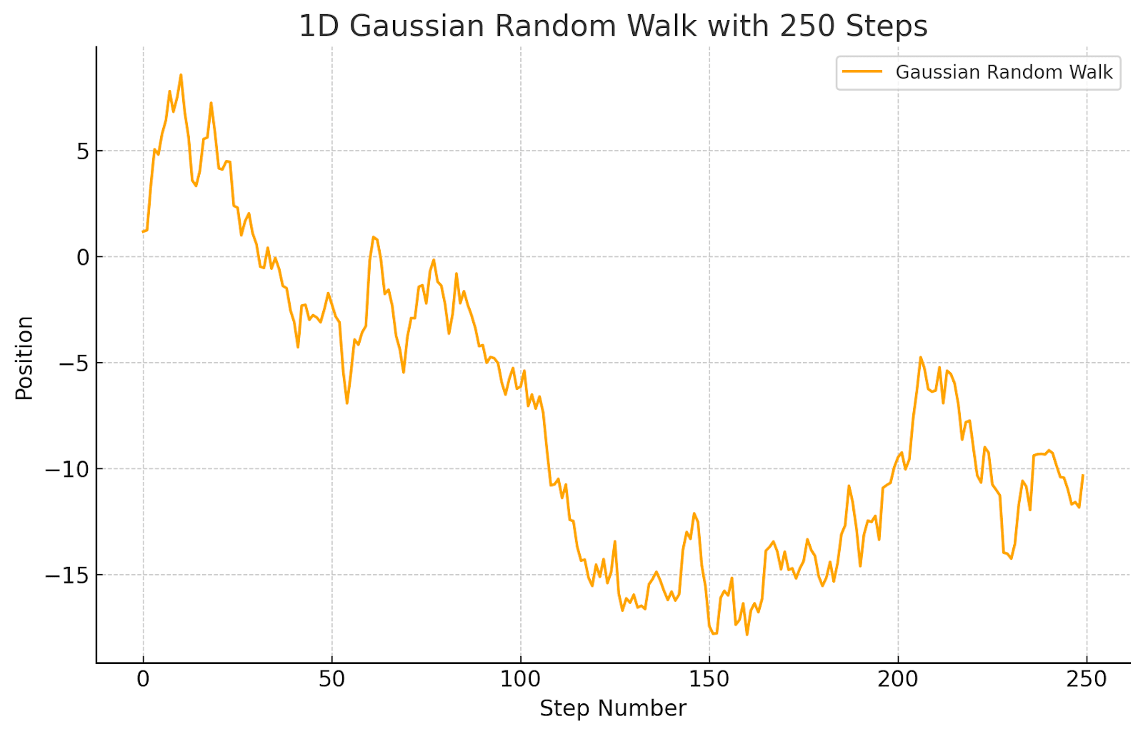
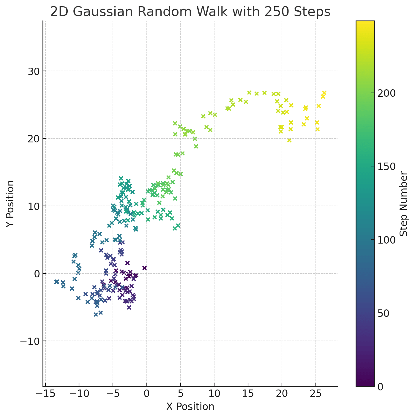
A random walk is the "null hypothesis" for any ordered collection of data with memory (a.k.a. any "time series" with memory). If you are looking at some learning process that updates state to state with some degree of stochasticity, seeing a random walk means that your update steps are random and you're not in fact learning. If you graph some collection of activations from layer to layer of a transformer (or any neural net architecture with skip connections -- this means that layer updates are added to "memory" from the previous layer) and see a random walk behavior, this means that you have in fact found no pattern in how the data gets processed in different layers. A random walk drifts over time, but ends up in a random place: you can't make any predictions of where it ends up (except predict the exact form of Gaussian randomness): 

Now one useful way that people use to find patterns in their data is make pictures. Since data in ML tends to be high-dimensional and we can only make 2-dimensional pictures^[1], we tend to try to plot the most meaningful or prediction-relevant data. A standard thing to do is to look at top PCA components: i.e., find the maximal-variance directions and look at how the data behaves in these directions. If we have generated some collection of possible interesting directions that reflect some maximally informative parameters that the internal data of an LLM tracks, we can examine their behavior one by one, but we expect to see the strongest form of the relevant behavior in the top PCA components. 

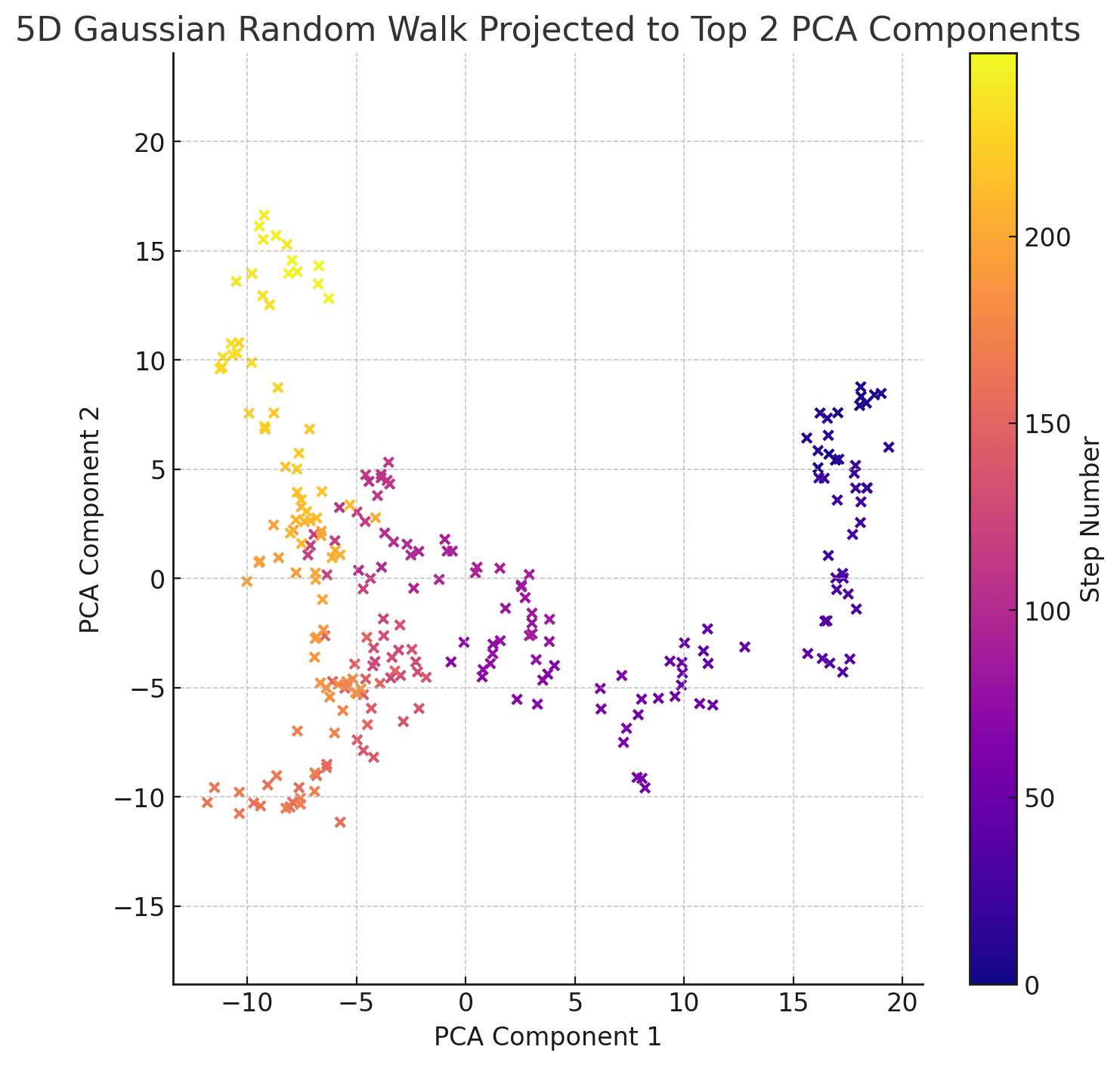
So if the top PCA components of a process with memory look like a random walk, that's even stronger evidence that we haven't found a pattern (at least a linear one). Here is a 5-dimensional random walk plotted to 2 dimensions via its top 2 PCA components: 

This still looks pretty random (with a random drift, as before).

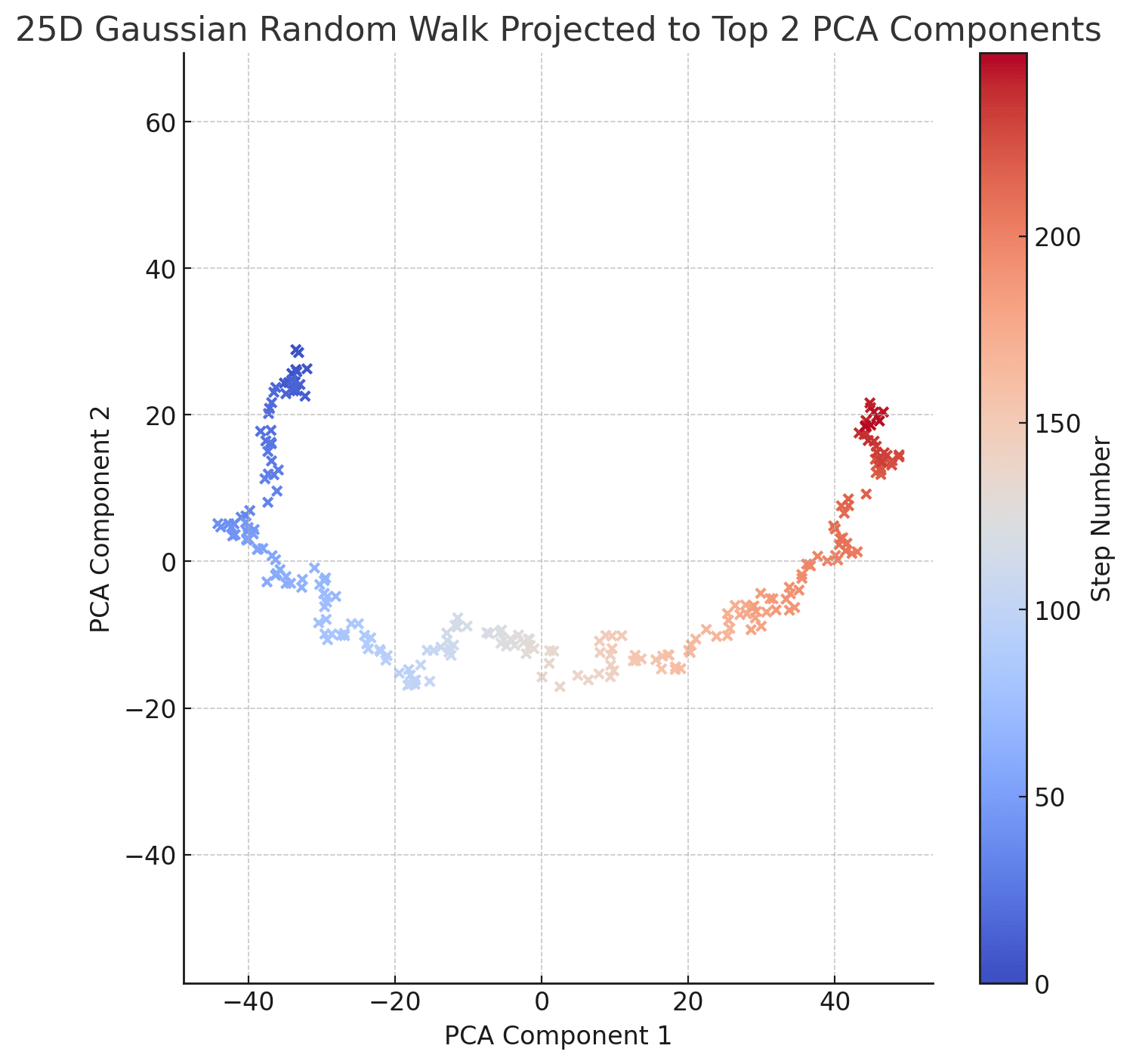
This is fun! Let's do the same thing with 250 points of a 25-dimensional random walk, plotted to their top 2 PCA:

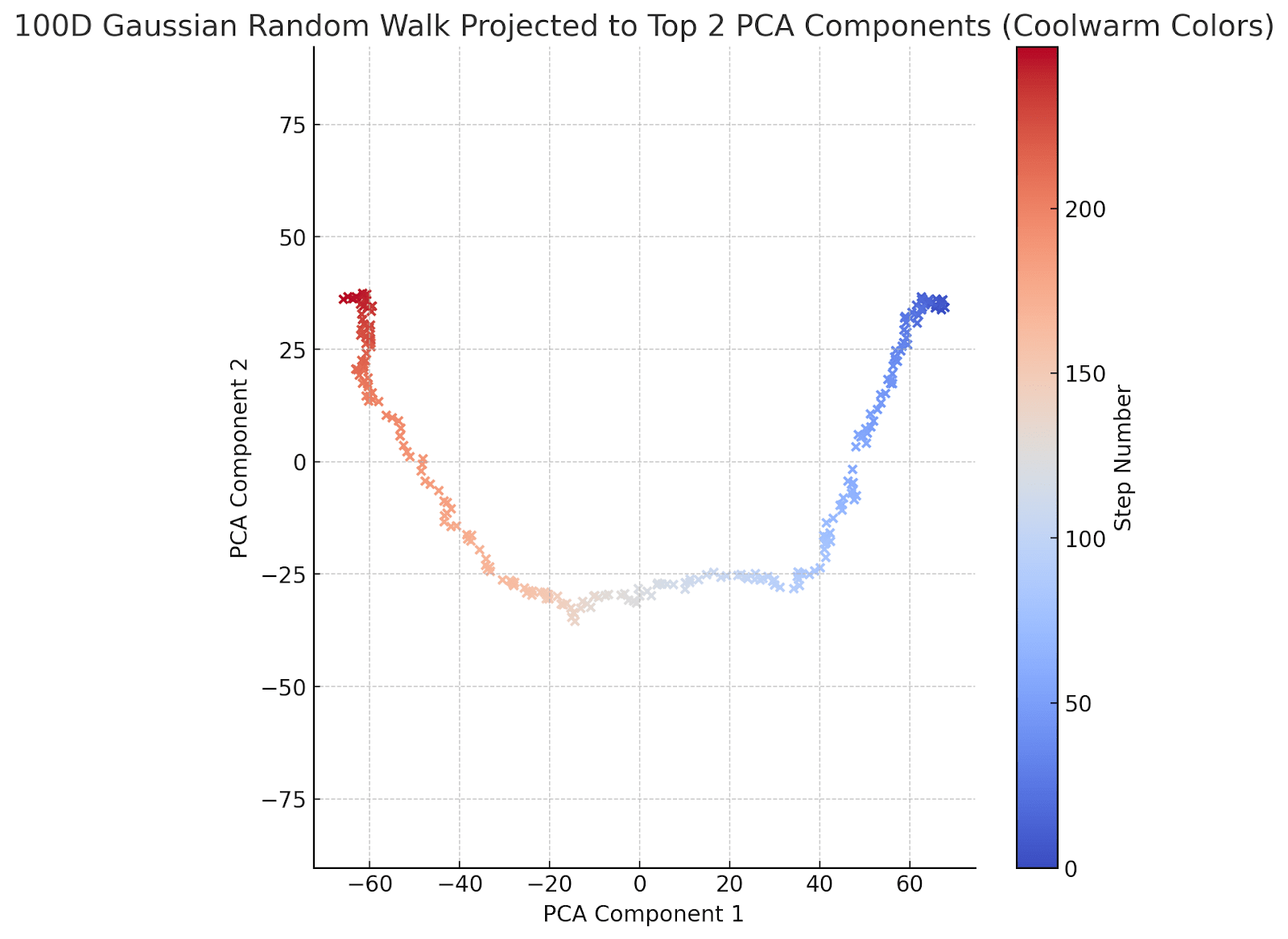
Hmm - something fishy is going on. Let's repeat with a 100-dimensional random walk:

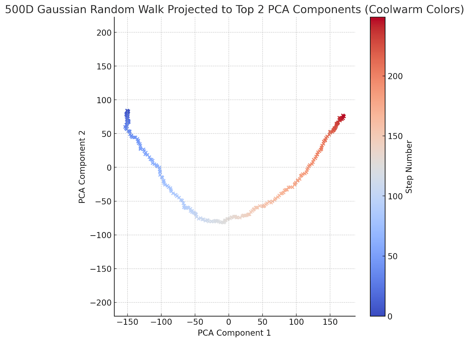
And a 500-dimensional random walk for good measure:

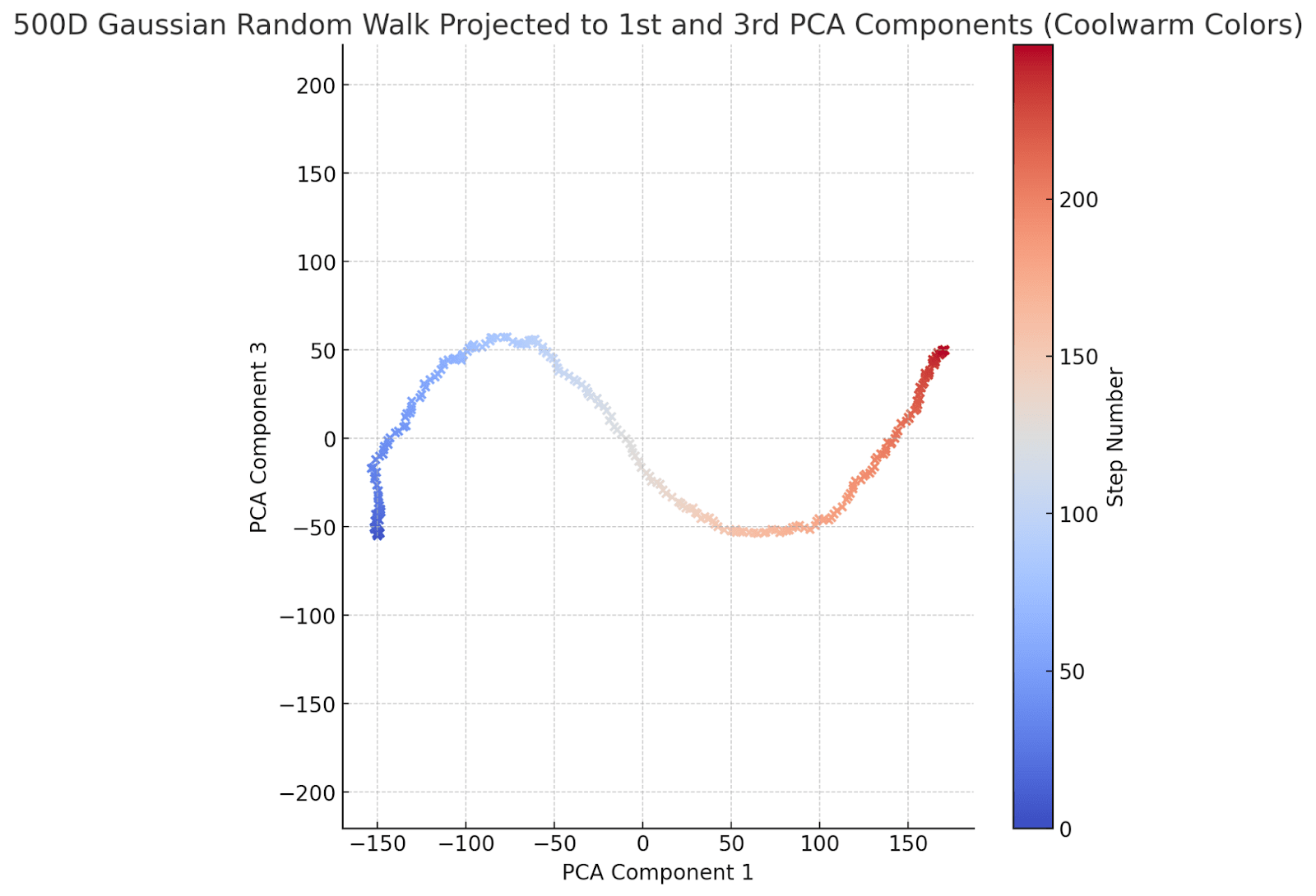
The character in the drunkard's walk has now obviously sobered up and decided where to go. To be fair, his y-coordinate movement is a bit indecisive: he ends up going down, then up -- but he purposefully walks from left to right. To help him along a bit, let's graph the first and 3d PCA components instead of the first and second:

Now he's indecisive in the y coordinate as well, but does end up in a new place in the y direction. 

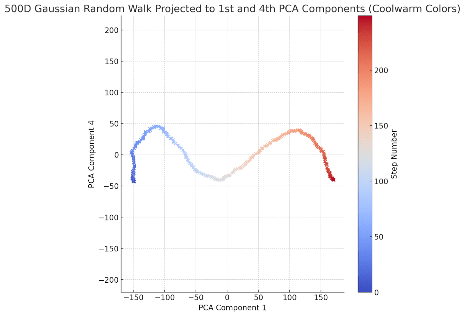
Just for fun, here is the 1st and 4th components:

This is very pretty! And I'll shortly explain how one can understand this. But first, notice that this captures a particularly frequent danger in statistical analysis of high-dimensional systems -- namely one of having too much control over the extracted data (related to, though not quite the same thing as, overfitting). When you have a lot of control, you can endow the bumbling drunkard with an arbitrary number of purposeful behaviors. This is all well and good when you are using this to generate pretty pictures or (as we'll do in a bit) talk about random matrices, but it's not great if you're framing an innocent drunkard for murder: "your honor, clearly he knew where he was going".

I experienced this phenomenon first-hand (acting as the "drunkard police") when Nina Panickssery and I were doing some followup work on our modular addition SLT project [LW · GW]^[2]. In doing this, we ran an SGLD sampler and just for fun, plotted the top two components. In the regime in which we were working (where all macroscopic measurements seemed to show the sampler to be unbiased), we saw strange pictures similar (though with a slightly more sophisticated geometric shape) to the random walk PCA above. We decided that there must be some secret extra directions in which the sampler remains biased (a.k.a. unstable -- the specific meaning of these words doesn't matter), though this sneaky direction doesn't interfere with any of the important large-scale parameters that we needed to sample (which we were quite sure, from several sources of inquiry, were behaving stably at the range we looked at). This wasn't the main point of the work, but it was a surprising thing that I remember pointing out as something to be careful to to some other people who were performing SGLD sampling. In other contexts, I've seen similar graphs of layerwise activations of neural networks graphed along such a PCA, with the curve behavior interpreted as capturing a pair of behaviors, one of which develops along layer depth and the other of which peaks, then goes back to baseline, as the layers go from early to middle to late. Later when I thought to perform this random walk PCA experiment, I experienced the familiar forehead-palm experience that I am learning to know and love in empirical research. 

So the main takeaway from this post is a warning: remember when you're doing something tricky and data-dependent to extract or graph your data, and make sure that you're not accidentally framing an innocent drunkard. (Note: if you look at more sophisticated random walks -- such as random walks with momentum, or slowly varying step size, etc., then you'll get a number of differently-shaped "pretty pictures" in the top PCAs. This can actually give usable insights if you're trying to explain a high-dimensional time series as a random process of a particular type, but if you're trying to find consistent macroscopic behaviors, then it's healthy to have a blanket suspicion of any pretty picture given by a PCA or any data extraction method that is data-dependent, or to at least put a bit of thought into some back-of-the-envelope degree-of-freedom computations to make sure the phenomenon you find isn't explained by overfitting.

Random matrices

Now let's finally think about why the pictures we see behave in this particular structured way. The key point, which is also the key class of insights in random matrix theory, is that eigenvalue-like invariants of random matrices have a significant amount of structure.

When modeling a random walk as a random process, we start with the matrix of random updates (i.e., the differences between subsequent points in the random walk): $$M_{upd}\sim N(0,1{)}^{d\times T}.$$ Here we assume that we're performing T steps of the random walk in d-dimensional space. Each step is vector in $R^d$ drawn from a Gaussian distribution, and since the updates are (by definition) uncorrelated, we have T independent draws. (Note: I'm not going to worry about normalization scales, since they'll all boil out into a single tunable constant at the end). 

Now each location in a random walk is $$x_t=M_1+M_2+\cdots +M_t,$$ where $M_i$ is the ith d-dimensional column of M. We can rewrite this using the $T\times T$ upper triangular "summation" matrix:

$$S=\left(\begin{array}{ccccc}1& 1& \dots & 1& 1\\ 0& 1& \dots & 1& 1\\ ⋮& ⋮& \ddots & ⋮& ⋮\\ 0& 0& \dots & 1& 1\\ 0& 0& \dots & 0& 1\end{array}\right).$$ Now the location matrix $X=x_1,x_2,\dots ,x_T$ is 

$$X=S\cdot M_{upd}.$$

Now the pictures we were drawing are obtained by:

• "centering" by subtracting the mean of each row of $X$ to get $X_{cent}$. This means multiplying on the left by another $T\times T$ matrix, $$C=I-\frac{1}{T}\left(\begin{array}{cc}1& \cdots \\ ⋮& \ddots ,\end{array}\right)$$ where the matrix on the left is the identity and the matrix on the right is the (normalized) matrix all of whose entries are 1.
• Finding the two top eigenvectors of the diagonal matrix
  $$X_{cent}^T{X}_{cent}=M_{upd}^T{S}^T{C}^{T}CS{M}_{upd}.$$
• Projecting columns of $X_{cent}=CS{M}_{upd}$ to the space spanned by these.

Now one can do pretty sophisticated random matrix theory to approximate this result, but there is a cheat that you can apply to get a stab at the "general behavior" for random walks in very large-dimensional spaces. Namely, in the limit where the dimension d is much larger than the number of steps T, one can simply assume that (up to rescaling), the random matrix of updates M_{upd} consists of T random orthogonal vectors. This is because of the most important result in high-dimensional spaces: 

The Johnson-Lindestrauss^[3] lemma: with very high probability, a collection of uniform Gaussian random vectors $v_1,\dots ,v_k$ in a very high-dimensional space is almost orthonormal. (With norm depending on the dimension and the variance of the Gaussians.)

I'm not saying exactly how to operationalize this, and indeed there are many operationalizations; here I'm just giving an intuition.

Once we observe this, we note that the projection we're looking at is independent of orthogonal changes of coordinates in the d-dimensional space^[4]. Thus if we were to really take the J-L lemma seriously and assume our update vector matrix $M_{upd}$ consists of a collection of orthonormal vectors (up to a fixed normalization rescaling), it follows that we can (up to a fixed scale) simply drop the random matrix $M_{upd}$, and work throughout with the deterministic matrix $CS$ that gets multiplied by $M_{upd}$. This means that (in the $d>>T$ limit), the elegant pictures we see are just the projections on the right of the matrix CS to its highest eigenvalues. Now we can check that $(CS{)}^{C}S$ is a nice matrix with incrementally changing entries (on a suitable scale), we should not be surprised that once the projections are worked out, they have the smooth form we see above. Note that what we used here isn't really random matrix theory, since we ultimately only looked at the singular vectors of a deterministic (namely, CS) rather than a random matrix.

Of course in most interesting examples, we're not working in the extreme $d>>T$ limit, and in fact the dimension d may be less than the number of datapoints T. In this case it's not longer legitimate to "overcommit" to the J-L lemma and model the datapoints as orthogonal. A full analysis would require more careful random matrix methods. Nevertheless, so long as the dimension d is not too much less than T, we should expect to still approximately notice the same large-scale behavior.

1. ^{^}

   Citation needed

2. ^{^}

   The followup work is currently unpublished, but I'm planning to write about something related to it later.

3. ^{^}

   Originally, this name was used for a more sophisticated extension of this insight to a statement about the way geometry changes under projection, but it has become standard to use this lemma as a catch-all for all related statements.

4. ^{^}

   To check this: if we are projecting a centered matrix M to a top principal value, the resulting T datapoints are Mv for v a top eigenvector of $M^{T}M$. Now if we write M'= MU for U an orthogonal matrix, then the vector $v^{\prime }=U^{-1}v$ is a top eigenvector of $(M^{\prime }{)}^T{M}^{\prime }$ (check this!). The corresponding projection is then $M^{\prime }{v}^{\prime }=MUU-1v=Mv$, i.e., doesn't change.

3 comments

Comments sorted by top scores.