Investigating the learning coefficient of modular addition: hackathon project

post by Nina Panickssery (NinaR), Dmitry Vaintrob (dmitry-vaintrob) · 2023-10-17T19:51:29.720Z · LW · GW · 5 comments

Contents

  Brief results
  Background
    Basics about the learning coefficient λ
    The Watanabe-Lau-Murfet-Wei estimate, ^λ
    Modular addition as a testbed for estimating λ
  Findings 
    Scaling behavior for generalizing networks
    (In)dependence on the number of circuits
    Random operations: scaling for memorization vs. generalization
    Dynamics and phase transition
None
5 comments

As our project at the Melbourne hackathon on Singular Learning Theory [? · GW] and alignment (Oct. 7-8), we did some experiments to estimate the learning coefficient of the single-layer modular addition task at a basin, an invariant that measures the information complexity (read: program length) of a fully trained neural net. 

We used the recent paper of Lau, Murfet, and Wei as our starting point; this paper estimates provides a stochastic estimate for the learning coefficient (which they denote $\hat{\lambda }$) via Langevin dynamics. The thermodynamic quantity measured by  $\hat{\lambda }$ is proven to asymptotically converge to the learning coefficient for idealized singular systems in a beautiful paper by Watanabe. 

All code for the experiments described can be found in this GitHub repository. 

Brief results

In our tests, we were pleasantly surprised to find that, for the task of modular addition modulo a prime $p$, the outputs of our implementation of Lau et al.'s SGLD methods are (up to a roughly constant small multiplicative error, less than a factor of 2) in robust agreement with the theoretically predicted results for an idealized single-layer modular addition network^[1]. 

Similar results have to date been obtained for a two-neuron network by Lau et al. and for a 12-neuron network by Chen et al. Our results are the first confirmation for medium-sized networks (between about 500 and 8,000 neurons) of the agreement between the estimate and the theoretical results. 

While our results are off by a small multiplicative factor from the theoretical value for a single modular addition circuit, we discover a remarkably exact phenomenon that perfectly matches the theoretical predictions, namely that the learning coefficient estimate is linear in $p$ for modular addition networks that generalize; this is the first precise scaling result of its kind.

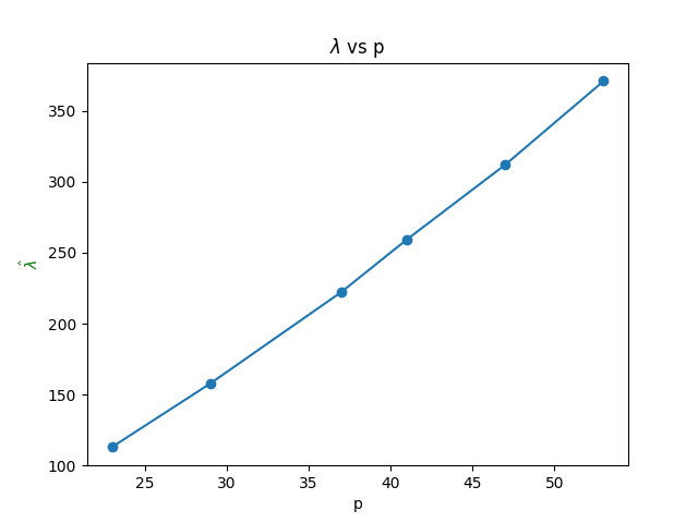
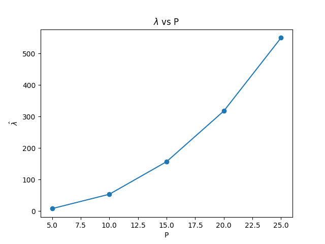
In addition, using the modular addition task as a test case lets us closely investigate the ability of the $\hat{\lambda }$ complexity estimate to differentiate generalization and memorization in neural networks: something that seems to be mostly new (though related to some of the phase transition phenomena in Chen et al.). We observe that while generalization has linear learning coefficient in the prime $p$, memorization has (roughly) quadratic growth in the prime $p$; this again exhibits remarkable agreement with theory.

The agreement with theory holds for multiple different values of the prime $p$ and multiple architectures. They also have appropriate behavior for networks that learn different numbers of circuits; a situation where other estimators of effective dimension, such as the Hessian-eigenvalue estimate, tend to overestimate complexity. 

Additionally, we show that the dynamic $\hat{\lambda }$ estimate^[2], i.e., the estimate during training, seems to track memorization vs. generalization stages of learning (this despite the fact that the $\hat{\lambda }$ estimate depends only on the training data). To see this, we use a slight refinement of the dynamical estimator, where we restrict sampling to lie within the normal hyperplane of the gradient vector at initialization, which seems to make this behavior more robust. 

Our dynamic results parallel some of the SGLD findings in Chen et al., which show that dynamic SGLD computations can sometimes notice phase transitions. We were pleasantly surprised to see them hold in larger networks and in the context of memorization vs. generalization. 

Overall, our findings update us to put more credence in the real-world applicability of Singular Learning Theory techniques and ideas. More concretely, we now believe that techniques similar to Lau et al.'s SGLD sampling should be able to distinguish different generalization behaviors in industry-scale neural networks and can be a part of a somewhat robust toolbox of unsupervised interpretability and control techniques valuable for alignment. 

Background

Basics about the learning coefficient $\lambda$

For an alternative introduction, see Jesse and Stan's excellent post [LW · GW] explaining the learning coefficient (published after we had written this section but following a similar approach).

The learning coefficient is a parameter associated with generalization. It controls the first-order asymptotic behavior of the question of "How likely is it that, given a random choice of weights, the loss they produce will be within ${\delta }_L$ of optimum". In other words, how easy is it to generalize the optimal solution to within ${\delta }_L$ accuracy. As ${\delta }_L$ goes to zero, this probability goes to zero polynomially, as an exponent of ${\delta }_L$, so 

${\text{Prob}}_{\text{Loss}<{\delta }_L}={\delta }_L^{d/2}+\text{lower order corrections.}$

(The $d/2$ instead of $d$ is there for technical reasons.) 

Such a term (usually defined in terms of the free energy: here ${\delta }_L$ is the temperature) occurs more generally in statistical physics (and has close cousins in quantum field theory) as the leading exponent in the "perturbative expansion." In the context of neural nets, the exponent $d$ it is called the learning coefficient or the RLCT ("real log canonical threshold," a term from algebraic geometry). 

The learning coefficient contains "dimension-like" information about a learning problem and can be understood as a measure of the effective dimension or "true dimensionality," i.e., the true number of weight parameters that need to be "guessed correctly" for a neural net to solve the problem with minimal loss. In particular, if a neural net is expanded by including redundant parameters that don't affect the set of algorithms that can be learned (e.g., because of symmetries of the problem), it can be shown that the learning coefficient does not change. Note that if the solution set to a machine learning problem is sufficiently singular (something we will not encounter in this post), the learning coefficient can be larger than the actual dimension of the set of minima^[3] and can indeed be a non-integer.

The Watanabe-Lau-Murfet-Wei estimate, $\hat{\lambda }$

In fact, the learning coefficient defined as a true asymptote only contains nontrivial information for singular networks, idealized systems that never appear in real life (just as it is not possible for two iterations of a noisy algorithm to give the exact same answer, so it is not possible for a network with any randomness to have a singular minimum or a positive-dimensional collection of minima). However, at finite but small values of temperature (i.e., loss "sensitivity," measured by ${\delta }_L$ as above), the problem of computing the associated free energy (and hence getting a meaningful generalization-relevant parameter at a "finite level of granularity") is tractable. 

The paper of Watanabe that Lau et al. follow gives a formula of this type. The result of that paper depends not only on the loss sensitivity parameter (called $\beta$, from the inverse temperature in statistical physics literature) but also on $n$, the number of samples. The formula gives an asymptotically precise estimate for the learning coefficient of the neural network on the "true" data distribution, corresponding to the limit as the number of samples n goes to infinity. As n goes to infinity, Watanabe takes the temperature parameter ${\delta }_L$ to zero as $\log \left(n\right)/n$. Lau et al.'s paper sets out to perform this measurement at finite values of $n$. 

Having a good estimator for the learning coefficient can be extremely valuable for interpretability: this would be a parameter that captures the information-theoretic complexity of an algorithm in a very principled way that avoids serious drawbacks of previously known approaches (such as estimates of Hessian degeneracy) and can be useful for out-of-distribution detection. More generally, the Singular Learning Theory [? · GW] program proposes certain powerful unsupervised interpretability tools that can give information about network internals, assuming the learning coefficient (and certain related quantities) can be computed efficiently.

Modular addition as a testbed for estimating $\lambda$

In Lau et al.'s paper, their SGLD-based learning coefficient estimate is applied to a tiny two-neuron network and also to an MNIST network, with promising results. We treat the modular addition network as an interesting intermediate case. Modular addition has to recommend itself the facts that: 

• It is a mechanistically interpreted network: we know its circuits, more or less how they are implemented by neurons, and how to isolate and measure them.
• We can cleanly distinguish networks that learn to generalize vs. networks that only memorize by looking at their circuits; moreover, we can "spoof" generalization by creating a network for learning a random commutative operation; this is a network that has the same memorization behavior as modular addition, but no possibility of generalization.
• We can count the number of generalization circuits a network learns and reason about how different circuits interact in the loss function and in somewhat idealized free energy computations. This allows us to compare the behavior of $\hat{\lambda }$ with respect to the number of circuits against other notions of complexity, for example, Hessian rank. 

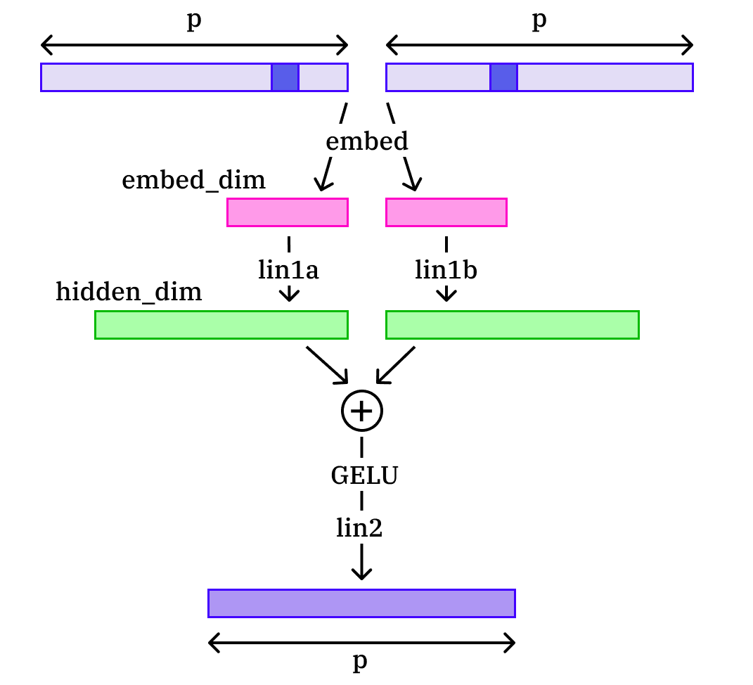
At the same time, being an algorithmically generated problem, modular addition has some important limitations from the point of view of SLT, which makes it unable to capture some of the complexity of a typical learning problem:

• The total number of possible data points for modular addition is finite (namely, equal to $p^2$ for $p$ the prime modulus), and the target distribution is deterministic. Thus, the learning coefficient only depends on a finite number of samples, which makes the asymptotic problem slightly (but not entirely) degenerate from the point of view of statistical learning theory.
• Even within the class of simple deterministic machine learning problems, the modular addition problem is highly symmetric; thus, it is possible for our empirical results to fail to generalize for less symmetric networks.
• The high number of possible output tokens compared to the maximal number of samples $p$ tokens compared to $p^2$ samples, for $p$ the modulus) may cause unusual behavior (Watanabe's results assume that the number of logits is small and the number of samples is asymptotically infinite).

Despite these limitations, we observed that (for an appropriate choice of hyperparameters) the Watanabe-Lau-Murfet-Wei estimate $\hat{\lambda }$ gives an estimate of the learning coefficient largely compatible with theoretical predictions. In addition, the estimates behave in a remarkably consistent and stable way, which we did not expect.

Findings 

We found that, for fully trained networks, SGLD estimates using Watanabe's formula give a good approximation (up to a small factor) of the theoretical estimate for the RLCT, both for the modular addition (linear in $p$, reasonably independent of the total number of parameters) and for the random network (quadratic in $p$). Moreover, it is independent of the number of atomic circuits, or "groks" (something we expect, in an appropriate limiting case, to be the case for the learning coefficient but not for other computations of effective dimension).

We also ran some "dynamical" estimates of  $\hat{\lambda }$  at unstable points along the learning trajectory of our modular addition networks. Here we observed that the $\hat{\lambda }$ estimates closely correlate to the validation (i.e., test) despite the fact that they are computed using methods involving only the training data. In particular, these unstable measurements "notice" the grokking transition between memorization and generalization when training loss stabilizes and test loss goes down.

Scaling behavior for generalizing networks

We ran the Watanabe-Lau-Murfet-Wei $\hat{\lambda }$-estimator algorithm on the following networks, and obtained the following results. We graph the $\hat{\lambda }$ estimate against each prime, averaged over five experiments. 

We found that estimates using Watanabe's formula gave a good approximation (up to a small factor) of the theoretical estimate for the RLCT, both for the modular addition and for the random network: 

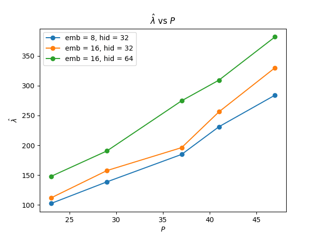
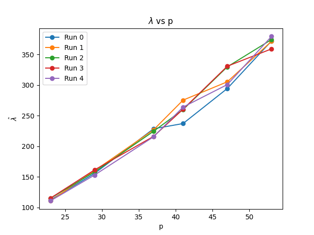
We observe that at a given architecture, our $\hat{\lambda }$ estimates are very close to linear, as would be theoretically predicted. 

In principle, the minimal effective dimensionality of a model with this architecture that solves modular addition is $4p$ (this will be elaborated on in a separate theory post deriving results about modular addition networks). However, we observe that the empirical scaling factor is very close to  $8p=2\times 4p$, double the result for a single circuit. A possible explanation for this result could be that, in the regime our models inhabit, the effective space of solutions consists of weight parameters that execute at least two simple circuits (all models we trained learned at least 4 simple circuits). 

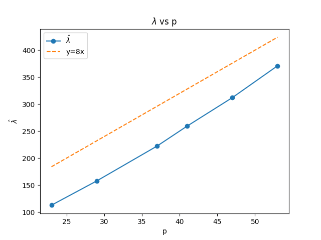
When starting the experiment, we were expecting extensive differences of more than an order of magnitude between the empirical and predicted values (because of the non-ideal nature of the real-life models and limiting points in our experiments). This degree of agreement between a relatively large and messy "real-world" measurement and an ideal measurement, as well as the near-linearity here, are by no means guaranteed and updated us a significant amount towards believing that the theoretical predictions of Singular Learning Theory match well to real-world measurements. 

We also repeat the experiment at various architectures, with the number of parameters different by a relatively large factor (our largest network is more than 3 times larger than our smallest network, and our intermediate network is asymptotically twice as big as the smallest one). Larger networks do have slightly higher $\hat{\lambda }$  , but the difference scales sub-linearly in network size, as we would expect from the true learning coefficient. 

Note that the primes we include are relatively small. While our architectures are efficient and always generalize (with close to 100% accuracy) for much larger primes, we empirically observe that the estimates for $\hat{\lambda }$ tend to be much better and less noisy when the fully trained network is very close to convergence (0 loss). Because of computational limitations, we use a relatively large learning rate (0.01) for a relatively small number of iterations. This results in worse loss at convergence for primes above 50; we conjecture that the near-linear behavior would continue to hold for much larger primes if we used more computationally intensive methods with a smaller learning rate and a larger number of SGD steps. 

(In)dependence on the number of circuits

The networks we train sometimes learn different numbers of independent generalizing circuits embedded in different subspaces (the existence of such circuits was first proposed by Nanda et al).

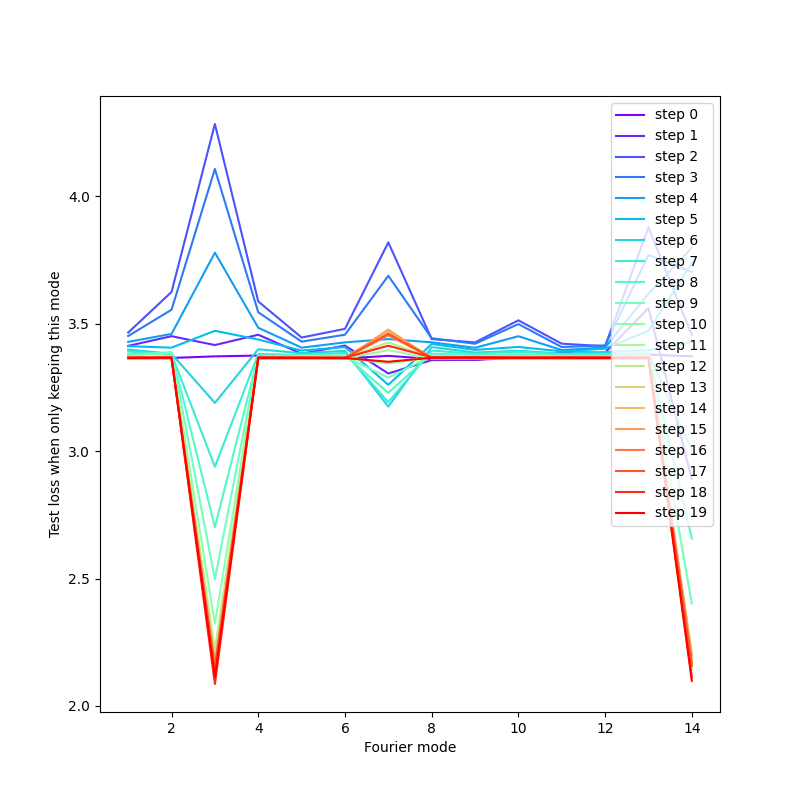
We can measure the number and types of circuits learned by a network, either by considering large outlier Fourier modes in the embedding space or (more robustly) by looking for near-perfect circles in "Fourier mode-aligned" two-dimensional projections of the embedding space^[4], as in the picture below

(We plan to later publish another post (on mechanistic interpretability tools for modular addition, in particular exactly distinguishing "pizza" from "clock" circuits), where these pictures will be explained more.)

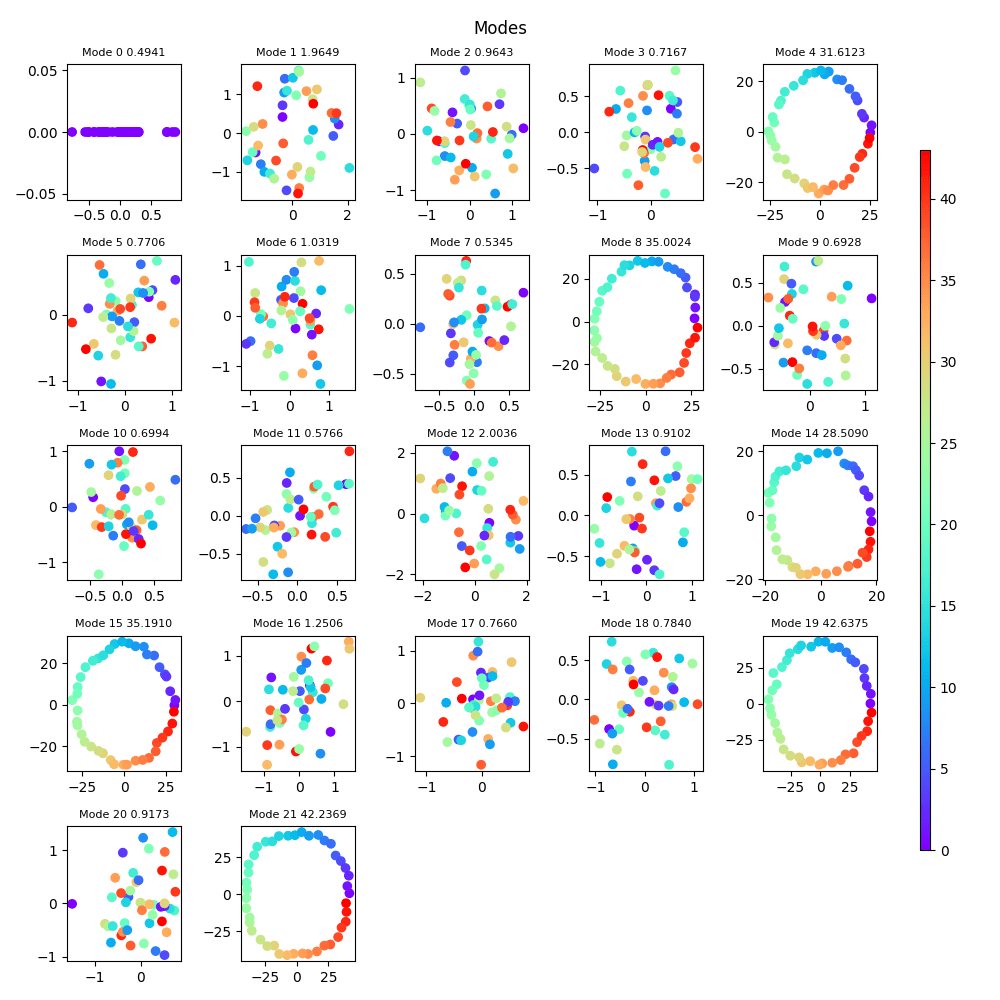
We observe in our experiments that the learning rate estimates do not seem to depend much on the number of circuits learned. For example, for the largest prime we considered, $p=53$, the number of circuits learned in different runs varied between 4 and 7 circular circuits, whereas the learning coefficients for all the networks were within about 10% of each other. This result is deceptively simple but quite interesting and somewhat surprising from a theoretical viewpoint. 

For example, when measuring the effective dimension of a network via Hessian eigenvalues, a network with more than one circuit will have either effective dimension 0 (because going along a direction corresponding to any circuit counts as generalizing) or effective dimension that depends linearly on the number of circuits (because a direction counts as generalizing only if it independently generalizes each of the circuits). The fact that neither of these behaviors is observed in our context can be motivated by the Singular Learning Theory framework. Indeed, we can treat the subspace in weight space executing each circuit (or perhaps a suitable small subset of circuits) as a separate component of a singular manifold of "near-minima." As the vector spaces associated to the different circuits are in general position relative to each other, the resulting singularity is "minimally singular"^[5]. This would mean that the RLCT at the singular point is equal to the RLCT along each of the individual components, which can be understood as an explanation for the observed independence result. However, we note that despite its explanatory robustness, this picture becomes more complicated when we zoom in since the loss for a multi-circuit network tends to be significantly better than the product of its parts. 

We plan to give an alternative explanation for the independence result involving a statistical model for cross-entropy loss that takes advantage of the ergodicity of multiplication modulo a prime. We flag here that we expect this independence to only hold in a "goldilocks" range of hyperparameter choices and, in particular, of the regularization constant (corresponding to the sizes of the circuits learned). A simplistic statistical model predicts at least three distinct phases here: one at a very small circuit size (corresponding to large regularization), where we expect the number of circuits to multiplicatively impact the learning rate. One at large circuit sizes (small regularization), where the learning rate estimate becomes degenerate, and one at an intermediate region, where the independence result we see is in effect.

Random operations: scaling for memorization vs. generalization

To compare our generalizing networks to networks with the same architecture, which only memorize, we ran the Watanabe-Lau-Murfet-Wei algorithm for a random commutative operation network. 

In order to get good loss for a memorization network, we need it to be overparametrized, i.e., the number of parameters needs to be above some appropriate $O\left(1\right)$ multiple of the total number of samples, in our case $p^2$. Because the number of parameters grows linearly in $p$, we get convergence to near zero loss only for small values of p. We note that since number-theoretic tricks like the Chinese Remainder Theorem are irrelevant for random operation networks, the values of p for this experiment do not need to be prime. Thus we run this experiment for multiples of 5 up to 40. Because of convergence issues and scaling pattern observation, we most trust our results in the short range of values between 5 and 25.

Note that this range overlaps with our list of primes only between 23 and 25; we would need to use larger networks (and probably, better learning convergence) to get reasonable values of $\hat{\lambda }$ above this range. For the range of values we consider, we observe a larger learning coefficient with a quadratic scaling pattern in $p$, compared to the linear linear for generalizing networks. 

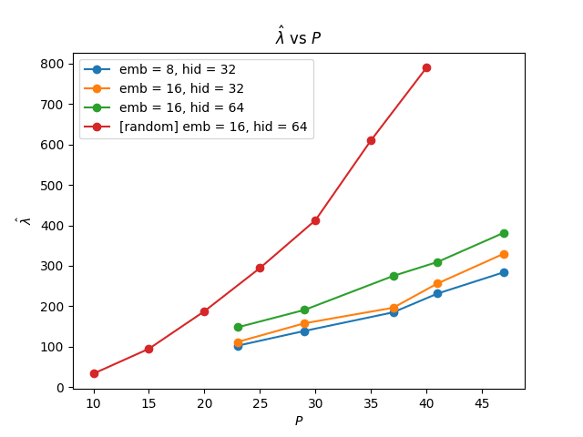
Remarkably, the diagram to p = 25 is almost exactly (up to a constant offset) equal to the number of memorizations, $0.8\cdot p^2$; here 0.8 is the fraction of the full dataset used for training. We also generated data for larger multiples of 5, up to 40. Here we see clearly that the memorizing network has higher learning rate than the generalizing network at the same architecture, but the quadratic fit becomes worse for $p>25$. We believe that we would recover quadratic fit for more values of p if we worked with a larger network. 

Dynamics and phase transition

Finally, we performed a dynamic estimate of the learning coefficient at various checkpoints during the learning process for generalizing networks. 

In this part of our results, we introduced some innovations to the methods of Lau et al. and Chen et al. (though we did not implement the "health-based" sampling trajectory sorting from the latter paper). Specifically, we got the best results with a temperature adjustment and with our implementation of unstable SGLD applied after restricting to the normal hyperplane to loss gradient.

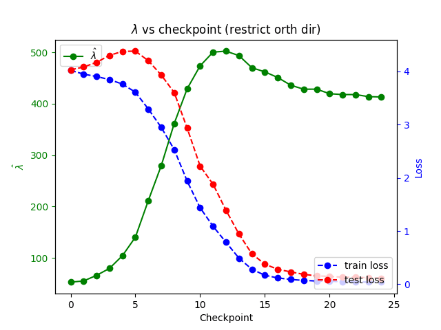
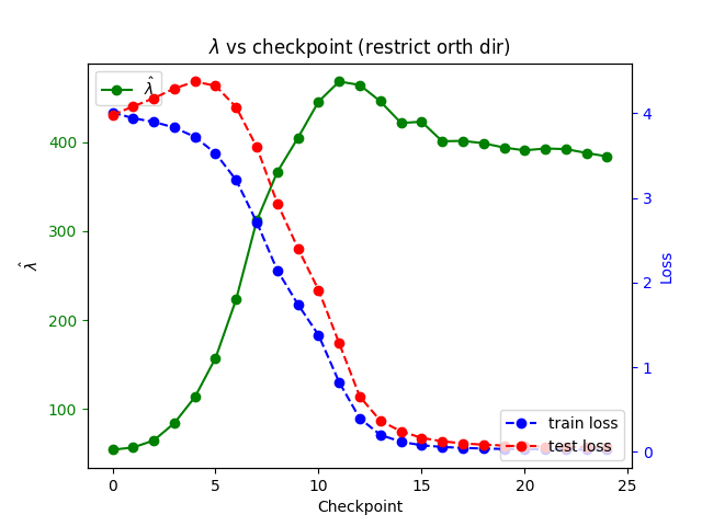
Here we observed that the unstable $\hat{\lambda }$ estimates closely correlate to the validation (i.e., test) despite the fact that they are computed using methods involving only the training data. In particular, these unstable measurements "notice" the grokking transition between memorization and generalization when training loss stabilizes and test loss goes down. (As our networks are quite efficient, this happens relatively early in training.)

1. ^{^}

   Note that Lau et al. also undertake an estimate of $\hat{\lambda }$ for a large MNIST network with over a million neurons. Here they find that the resulting value for $\hat{\lambda }$ is correlated with the optimization method used to train the network in a predictable direction and thus captures nontrivial information about the basin. However, the theoretical value of $\hat{\lambda }$ is not available here, and the SGLD  algorithm fails to converge; thus, this estimate is not expected to give a faithful value of the learning coefficient in this case 

2. ^{^}

   Note that the dynamic $\hat{\lambda }$ estimator attempts to apply a technique designed for stable points (i.e., local minima) to points that are not local minima and have some instability, sampling, and ergodicity issues, even with our normal-to-gradient restriction refinement. In particular, they (much more than estimates at stable points) are sensitive to hyperparameters. Thus these unstable $\hat{\lambda }$ measurements do not currently have an associated exact theoretical value and can be thought of as an ad hoc generalization of a complexity estimate to unstable points. Nevertheless, we find that at a fixed collection of hyperparameters, these estimates give consistent results and look similar across runs, and we see that they contain nontrivial information about the loss landscape dynamics during learning.

3. ^{^}

   An intuition for this is that very singular loss functions (i.e., functions that have many higher-order derivatives equal to zero) are associated with very large basins, which are large enough to "fit in extra dimensions worth of parameters."

4. ^{^}

   The two-dimensional subspace of the embedding space $R^{\text{embed\_dim}}$ associated with the kth Fourier mode is the space spanned by the sin and cos components of the k-frequency discrete Fourier transform. Note that these spaces are not necessarily linearly independent for different modes but are independent for modes that learn a circuit.

5. ^{^}

    This is meant in an RLCT sense. In algebraic geometry language, a function f on weight space $R^n$ is minimally singular if there exists a smooth analytic blowup $X\to R^n$ such that in local coordinates on X, f is a product of squares of coordinate functions. In this language, if we have c circuits associated to vector subspaces $C_1,\dots ,C_c$ in weight space, an "idealized" function with minima on k-tuples of circuits is the function 

   $f\left(w\right)={\sum }_{S\subset \{1,\dots ,c\},|S|=c-k+1}{\prod }_{i\in S}\text{dist}(w,C_i{)}^2$

   for $S$ running over $c-k+1$-element subsets and $\text{dist}(w,C_{i_j})$ the L2 distance from a weight to the corresponding subspace. It is easy to check that the resulting singularity is minimally singular.

5 comments

Comments sorted by top scores.