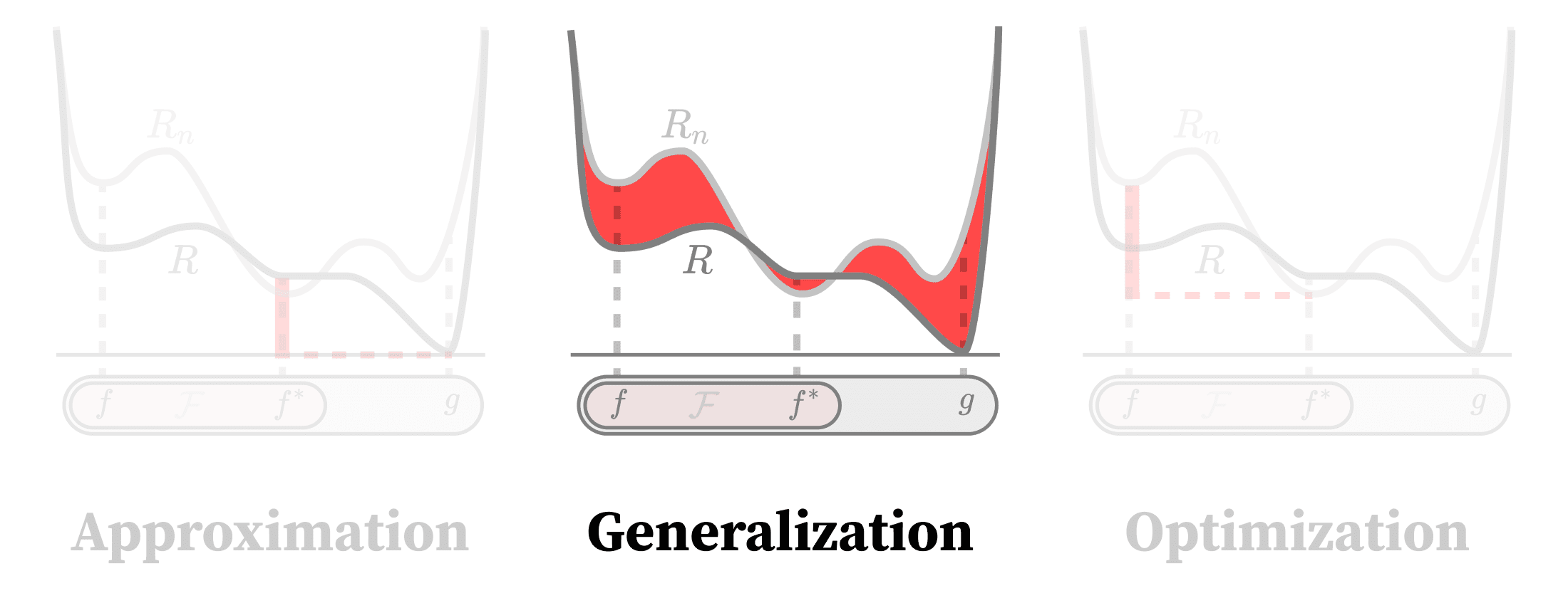
Generalization, from thermodynamics to statistical physics

post by Jesse Hoogland (jhoogland) · 2023-11-30T21:28:50.089Z · LW · GW · 9 comments

Contents

  Summary
  Introduction
    Outline
  Measuring "generalization"
    The generalization error
    Derived generalization metrics
    Bayesian generalization metrics
  Bounding generalization
    Global vs. Local
    Dataset-dependence
    Flavors of generalization bounds
    Named families of bounds
      Uniform convergence
      Probably Approximately Correct (PAC)
      Mean Approximately Correct (MAC)
      PAC Bayes
  Measuring "complexity"
    Model-class complexity
      Vapnik-Chervonenkis (VC) dimension
      Rademacher complexity
      Covering numbers
    Single-model complexity
      Margins
      Minimum flatness/sharpness
      Algorithmic stability and robustness
    Model-subclass complexity
      Information-theoretic metrics
      Compressibility
      The free energy / stochastic complexity
      Learning coefficient
      Singular fluctuation
      Multiplicity
      Weight norm
  Thermodynamics of generalization
    Internal model selection
    Why model subclasses
    Why neural networks generalize
    How neural networks generalize
    Future research
None
9 comments

Summary

In 2018, Zhang et al. showed that deep neural networks can achieve perfect training loss on randomly labeled data.

This was a Big Deal.

It meant that existing generalization theory couldn't explain why deep neural networks generalize. That's because classical approaches to proving that a given model class (=neural network architecture) would generalize involved showing that it lacks the expressivity to fit noise. If a model class can fit noise arbitrarily well, the resulting bounds break.

So something needed to change.

Evidently, you can't prove tight generalization bounds for entire model classes, so theorists turned to studying generalization bounds for individual models within a model class. If you can empirically show that a model's performance doesn't change substantially when you perturb it (by adding noise to the inputs, weights, training samples, etc.), then you can theoretically prove that that model will generalize to new data.

As a result, the bounds have gotten tighter, but they're still not exactly flattering.

What's really needed is a secret third thing. It's not about either model classes or individual models but about model subclasses. While the model class as a whole may be too complex to obtain tight generalization bounds, individual subclasses can achieve an optimal trade-off between accuracy and complexity. For singular Bayesian learning machines, this trade-off happens automatically.

This more or less answers why models are able to generalize but not how they do it.

Singular learning theory (SLT) provides one possible path towards understanding the how of generalization. This approach is grounded in the geometry of the loss landscape, which in turn is grounded in the symmetries of the model class and data. If this direction pans out, then learning theory is posed for a revolution analogous to the transition between thermodynamics and statistical physics.

Introduction

The central aim of classical learning theory is to bound various kinds of error: in particular, the approximation error, generalization error, and optimization error.

In the previous post in this series [LW · GW], we looked at the approximation error, which measures the performance of a model class's hypothetically optimal model. If your model class isn't expressive enough to do a reasonable job of modeling the data, then it doesn't matter that your model generalizes to new data or that your learning process actually reaches that optimum in practice.

In this post, we'll look at bounding the generalization error, which measures how well a model $f_w\in F$ parametrized by $w\in W$ transfers from a finite training set to additional samples drawn from the same distribution.  We won't cover the related question of out-of-distribution generalization, which asks how a model will perform on data from a different distribution. 

Last time, we started to see that approximation and generalization could not be separated in practice. Here, we'll see the same holds for generalization and optimization. SLT and many other strands of generalization theory point to a deep relation, which views generalization in nearly dynamical terms involving changes to probability distributions. 

In the next post in this sequence, we'll examine the optimization error, which measures how close learning processes get to global optima. Coming at the connection with generalization from the other direction, we'll view optimization in quasistatic terms as a process of selecting among qualitatively distinct generalization strategies. 

This is mainly based on lecture notes by Telgarsky (2021), a recent monograph by Hellström et al. (2023), and Watanabe (2009, 2018).

Outline

This is a self-contained introduction to generalization theory, as developed in three different schools of learning theory: classical learning theory, deep learning theory, and singular learning theory. There's a lot to cover:

• Measuring "generalization" — First, we treat the question of how to quantify generalization, and how this differs between the paradigms of empirical risk minimization and Bayesian inference. 
• Bounding generalization — Next, we look at the different kinds of bounds learning theorists study. This will include classical approaches like uniform convergence and Probably Approximately Correct (PAC) learning, as well as more modern approaches like PAC Bayes.
• Measuring "complexity" — Then, we'll cover the three different types of complexity measures that show up in these bounds: model-class complexity, single-model complexity, and model-subclass complexity. These roughly correspond to the different perspectives of classical learning theory, deep learning theory, and singular learning theory, respectively. 
• Thermodynamics of generalization — Finally, we'll examine the model-subclass complexity measures from a thermodynamic point of view. This raises the natural question: what would a statistical physics of generalization look like and what might we learn about how neural networks generalize?

Measuring "generalization"

The generalization error

To recap [? · GW], classical learning theory is primarily grounded in the paradigm of Empirical Risk Minimization (ERM). ERM is a story about two kinds of risk. 

The empirical risk $R_n$ is what you might recognize as the "training loss",

$$R_n\left(f_w\right):=\sum _{i=1}^n\ell \left(f_w\right(x_i),y_i),$$

where the average is taken over the $n$ samples in your dataset $D_n=\left\{\right(x_i,y_i){\}}_{i=1}^n$.^[1] Learning theorists maintain a sensible distinction between the individual-sample "loss" function $\ell$ and the average-loss "risk" $R_n$.

The population risk (or "true" risk) $R$ is the expectation of the loss over the true distribution $q(x,y)$ from which the dataset is drawn:

$$R\left(f_w\right):=E_{q(x,y)}\left[\ell \right(f_w\left(x\right),y\left)\right]=\int \ell \left(f_w\right(x),y)q(x,y)dxdy.$$

In its broadest form, generalization is the question of how a model transfers from a finite dataset to new data. In practice, learning theorists study the generalization error (or generalization gap) $G_n\left(f_w\right)$, 

$$G_n\left(f_w\right):=|g_n\left(f_w\right)|:=|R\left(f_w\right)-R_n\left(f_w\right)|,$$

which addresses a more narrow question: how far apart are the empirical risk and population risk?

Derived generalization metrics

The generalization error, $G_n$, is a function of both the learned model $f_w$ and dataset $D_n$, so by taking expectation values over data, weights, or both, we derive a family of related generalization metrics.

The relevant distributions include:

• $p\left(w|D_n\right)$: the "learning algorithm", some mapping from a dataset to weights. If we're using a deterministic algorithm, this becomes a delta function. In Bayesian learning, this is the posterior. For neural networks, think of the distribution of final weights over initializations and training schedules for a set of fixed optimizer hyperparameters.
• $q\left(D_n\right)={\prod }_{i=1}^{n}q(x_i,y_i)$: the true probability of the dataset. We're assuming samples are i.i.d.
• $p(w,D_n)=p\left(w|D_n\right)q\left(D_n\right)$: the joint distribution over learned weights and datasets.

From these distributions, we obtain:^[2]

• $E_{p(w,D_n)}\left[G_n\right(f_w\left)\right]$: the average generalization error over learned weights and datasets.
• $E_{q\left(D_n\right)}\left[G_n\right(f_w\left)\right]$: the average generalization error over datasets for a fixed model $f_w$.
• $E_{p\left(w|D_n\right)}\left[G_n\right(f_w\left)\right]$: the average generalization error over learned weights for a fixed dataset $D_n$.
• $G_n\left(E_{p\left(w|D_n\right)}\right[f_w\left]\right)$: the generalization error for the average prediction made by the learned models for a fixed dataset.

And so on.

Bayesian generalization metrics

In a Bayesian setting, we replace the deterministic prediction $\hat{y}=f_w\left(x\right)$ with a distribution $p(y|x,w)$, which induces a likelihood $p\left(D_n|w\right)={\prod }_{i=1}^{n}p(y_i|x_i,w)q\left(x_i\right)$. Under certain assumptions, empirical risk minimization maps onto a corresponding Bayesian problem, in which the empirical risk is the negative log likelihood (up to a constant).^[3] 

The Bayesian learning algorithm is the posterior,

$$p\left(w|D_n\right)=\frac{p\left(D_n|w\right)\phi \left(w\right)}{p\left(D_n\right)}.$$

But we're not just interested in updating our beliefs over weights — we also want to use our new beliefs to make predictions. Theoretically, the optimal way to do this is to average novel predictions over the ensemble of weights, weighing each machine according to their posterior density. This yields the predictive distribution,

$$p(y|x,D_n)=E_{p\left(w|D_n\right)}\left[p\right(y|x,w\left)\right]=\int p(y|x,w)p\left(w|D_n\right)dw.$$

In practice, evaluating these kinds of integrals is intractable. A more tractable alternative is Gibbs estimation, where we draw a particular choice of weights $w^{\prime }\sim p\left(w|D_n\right)$ and make predictions using the corresponding model $p(y|x,w^{\prime })$. This procedure is closer to the kind of paradigm we're in with neural networks: the model we train is a single draw from the distribution of final weights over different initializations and learning schedules. 

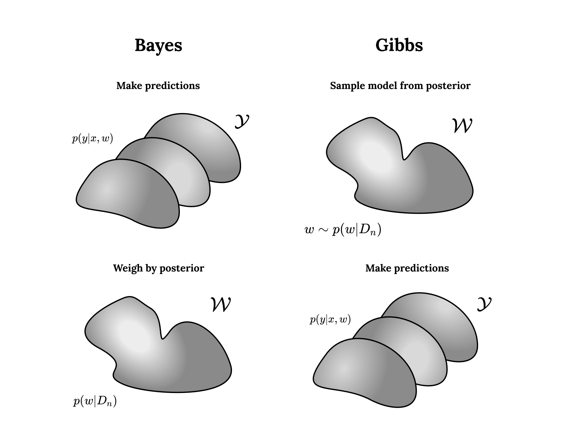
Predicting according to either the predictive distribution or Gibbs estimation respectively yields two different kinds of generalization error:

• The Bayes generalization error is the KL divergence between the true distribution and the predictive distribution:

$$\begin{array}{cc}{G}_n^B:=& D_{KL}\left(q\right(y|x)\parallel p(y|x,D_n\left)\right),\\ =& E_{q\left(y|x\right)}\left[\log \frac{q\left(y|x\right)}{E_{p\left(w|D_n\right)}\left[p\right(y|x,w\left)\right]}\right].\end{array}$$

• The Gibbs generalization error is the posterior-averaged KL divergence between the true distribution and the model $p(y|x,w)$:

$$\begin{array}{cc}{G}_n^G:=& E_{p\left(w|D_n\right)}\left[D_{KL}\right(q\left(y|x\right)\parallel p(y|x,w)\left)\right],\\ =& E_{p\left(w|D_n\right)}\left[E_{q\left(y|x\right)}\left[\log \frac{q\left(y|x\right)}{p(y|x,w)}\right]\right].\end{array}$$

Making predictions for a given model and sampling according to the posterior are non-commutative — it's not possible to move the expectation value in or out of the above logarithm without changing the result. Thus, we get two different approaches to prediction and two different kinds of generalization error. 

Bounding generalization

When deriving generalization bounds, we have to decide not only which generalization metric to bound but also how to bound it. There are three main decisions:

1. "Global" or "local"? Do you want the results to hold over the entire set of weights or for a particular choice of weights?
2. Dataset-dependent or -independent? Do you want the results to hold for your particular set of samples or across all possible choices of datasets?
3. Uniform, average, or probabilistic? Do you want the bound to hold always, on average, or with some minimum probability?

Global vs. Local

The first and most important question is whether to bound generalization error over the entire model class or only for a particular model. Classical learning theory takes a global approach. Modern deep learning theory takes a more local approach. Singular learning theory suggests a third mesoscopic approach that obtains generalization bounds for model subclasses.

Global bounds. The global approach is a worst-case approach. The upper bound has to hold for all models, so it's only as tight as your worst-generalizing model. Finding these worst cases typically involves asking how well the model class can fit random noise. A model trained on purely random noise can't generalize at all because there's no signal, so fitting random noise perfectly means worst-case generalization error is terrible. This turns generalization into a question of expressivity, which is operationalized by complexity metrics like the VC dimension, the Rademacher complexity, and covering numbers. 

Because neural networks often can fit noise perfectly, they're highly complex according to these measures, and the resulting bounds become vacuous: they trivially predict that test error will be less than 100%. 

The reason we observe good generalization in practice is that not all models within a class are equally complex. For example, the success of weight-pruning shows that many weights can safely be set to zero and eliminated. Thus, average generalization can be very different from worst-case generalization. 

Local bounds. Instead of studying how well a model class can express noise, you can study how robust a specific model is to noise — noise applied to the inputs (margin theory), noise applied to the weights (minimum sharpness/flatness, compression theory), or noise applied to the training samples (algorithmic stability & robustness). To obtain a generalization bound, it's possible to exchange these kinds of empirical robustness-to-noise for predicted robustness-to-new-data. 

Though these results have led to real improvements, the bounds remain far too loose to explain large real-world models. Even for MNIST, the best upper bounds for % test error are an order of magnitude larger than what we actually observe in state-of-the-art models. Will progress eventually catch up, or do these limitations reflect a more fundamental problem with this approach?

Mesoscopic bounds. Instead of studying how much a single model react in response to noise, you can study how the distribution of learned models react in response to noise. With a change of perspective, this turns studying generalization into a question of comparing model subclasses. 

This point of view is already implicit in the areas of deep learning theory that obtain generalization bounds involving weight norm, compression, minimum sharpness/flatness, and various information-theoretic quantities. It is made explicit in singular learning theory, which proposes a set of canonical observables for studying model complexity and generalization, such as the learning coefficient, the singular fluctuation, and multiplicity. For idealized Bayesian learners, SLT predicts the values (not just upper bounds) of both Bayes and Gibbs generalization error in the large-data limit. 

Dataset-dependence

A second question is whether to bound generalization error for the given dataset or across the distribution of possible datasets. Practically, we only have a single dataset and want to understand how models will generalize for that particular dataset. Theoretically, it's usually easier to marginalize out the dependence on a specific dataset. 

Marginalizing the dataset is often justified on the grounds that we're more interested in how the model performs in the limit of large amounts of data. In these limits, the influence of any single data point vanishes. However, this assumption may not hold in situations where the distributions have fatter tails like RL.

Flavors of generalization bounds

The last question is mostly aesthetic: how do we dress up our bounds? Since generalization is made up of both data and weights, this breaks down into two subquestions: how to dress up the bound over data and how to dress up the bound over weights? 

Uniform bounds. The strongest kind of bounds are ones that holds uniformly over the model class, that is, bounds involving universal quantifiers:

$$G_n\left(f_w\right)<ϵ,\forall w\in W$$

This is defined relative to weights because we're rarely interested in bounds that hold uniformly over datasets. Except for trivial distributions, there are always pathological draws of data that will exhibit poor generalization. 

Probabilistic bounds. Weaker (in the sense that they don't always hold) but often tighter (the upper bound is lower) are bounds that hold "in probability":

$$P\left(G_n\right(f_w)<ϵ)>1-\delta .$$

Though one could formulate a probabilistic bound relative to the distribution over weights, in practice, these bounds are always defined relative to the distribution over data. 

Expectation bounds. Weaker yet tighter still are bounds that hold "in expectation." These are bounds that hold after taking an expectation value over weights/datasets:

$$E\left[G_n\right(f_w\left)\right]<ϵ.$$

Unlike uniform bounds that are usually reserved to weights and probabilistic bounds that are usually reserved to data, expectation bounds treat weights and data on more equal footing. 

Combining bounds. Given these choices, it's possible to mix and match. Because these operations are non-commutative, you can swap the order to double the bounds. Vary the choice of underlying probability distribution, and the horrible profusion of different generalization bounds grows further. To simplify matters somewhat, it's often possible to transform bounds in one format to another. 

Named families of bounds

Many of the particular combinations of choices for how and what to bound have dedicated names. Unfortunately, these names are neither exhaustive nor exclusive nor consistent.

A few of the more important ones:

1. Uniform convergence: bound $G_n$ in probability over draws of a dataset and uniformly over all possible choices of model $w\in W$ and for all possible choices of data-generating distribution $q(x,y)$.
2. Probably Approximately Correct (PAC): bound $G_n$ in probability over draws of the dataset $D_n$ for a particular data-generating distribution and uniformly over the model class.
3. Mean-Approximately Correct (MAC): bound $G_n$ in expectation over the joint distribution. In other words, bound $E_{p(w,D_n)}\left[G_n\right]$.
4. PAC Bayes: bound $E_{p\left(w|D_n\right)}\left[G_n\right]$ in probability over draws of the dataset.
5. Single draw: bound $G_n$ in probability over $p(w,D_n)$.
6. Mean-hypothesis bounds: bound $G_n\left(E_{p\left(w|D_n\right)}\right[f_w\left]\right)$.

In principle, the qualitative shape of the bound is orthogonal to the question of which specific quantities show up in the bounds. In practice, the distinction often gets muddled. For example, "PAC Bayes" refers both to the general idea of a PAC-style bound on $E_{p\left(w|D_n\right)}\left[G_n\right]$ and to the specific idea of bounds that depend on a KL divergence between the posterior and prior. So it goes. 

Uniform convergence

Uniform convergence is the most classical of the classical approaches to generalization theory. The term comes from analysis, where we say that a sequence of functions $f_n$ converges uniformly to a limiting function $f$ if for every $ϵ>0$ there exists a natural number $N$ such that for all $n>N$ and for all inputs $x$,

$$|f_n\left(x\right)-f\left(x\right)|<ϵ.$$

In learning theory, we're interested in the empirical risk converging uniformly to the true risk, which means that the difference between the empirical risk and true risk becomes arbitrarily small for every model provided you have enough data (Hellström et al. 2023, Shalev-Shwartz et al. 2010):

$$\underset{q\in Q}{sup}{E}_{q\left(D_n\right)}\left[\underset{w\in W}{sup}{G}_n\right(f_w\left)\right]\stackrel{n\to \infty }{⟶}0.$$

Confusingly, the expectation value over data can be replaced by a probabilistic bound. The important bit of uniform convergence is that it is a form of "worst-case" analysis: you obtain a bound that holds uniformly both across all possible models in the model class and across all possible choices of data distribution $q\in Q$.

There are two problems with uniform convergence from the perspective of deep learning:

1. Generalization is not uniform across the model class. Given two models with the same performance on the training dataset, one may nevertheless generalize better than the other on new data.
2. Generalization is not uniform across data-generating distributions. The fact that neural networks can generalize well when trained on real-world datasets and generalize poorly when trained on random data suggests our bounds should be sensitive to the choice of data distribution.

Probably Approximately Correct (PAC)

The PAC-learning framework (Valiant 1984) addresses the second weakness of uniform convergence bounds: PAC-style bounds are defined relative to some fixed data distribution. The bounds still hold uniformly over the model class but are now defined in probability over data:

$$P_{q\left(D_n\right)}\left[\underset{w\in W}{sup}{G}_n\right(f_w)<ϵ]\ge 1-\delta .$$

Your model class will "probably" (with probability at least $1-\delta$) be "approximately correct" (with generalization error less than $ϵ$).

In particular, learning theorists then try to relate $ϵ$ and $\delta$ to each other and other hyperparameters like the number of parameters $d$, the number of samples $n$, the weight norm $|w|$, etc. Then, you can invert the relation to figure out how large you should make your model and how many samples you need to obtain a desired error with a desired probability.

For example, if the model class $F$ is finite, then, it satisfies the PAC bound so long as the sample size obeys

$$n\ge \frac{1}{2{ϵ}^2}(\log 2|F|+\log \frac{1}{\delta }).$$

The minimum $n$ that satisfies a bound of this kind is called the sample complexity.

Historically, much of the work in PAC-style generalization theory has looked like trying to replace the $\log 2|F|$ term above with a suitable finite complexity measure when the model class becomes infinite (see comments by Telgarsky 2021).

Mean Approximately Correct (MAC)

PAC-learning is more relaxed than uniform convergence, but it's still a worst-case approach where the bounds have to hold across the entire model class. The relaxation is in the data distribution. Instead, we can consider an average-case bound that holds on expectation over learned models and different draws of the data,

$$E_{p(w,D_n)}\left[G_n\right(f_w\left)\right]<ϵ.$$

A practical example is the following bound,

$$\left|E_{p(w,D_n)}\right[g_n\left(f_w\right)\left]\right|\le \sqrt{\frac{I(w\parallel D_n)}{2n}},$$

in terms of the mutual information between weights and data

$$I(w\parallel D_n)=D_{KL}\left(p\right(w,D_n)\parallel p(w\left)q\right(D_n\left)\right).$$

PAC Bayes

PAC Bayes (McAllester 1999, Shawe-Taylor and Williamson, 1997) keeps the expectation value over weights but swaps the expectation value over data with a probabilistic bound over data:

$$P_{q\left(D_n\right)}\left[E_{p\left(w|D_n\right)}\right[G_n\left(f_w\right)]<ϵ]<1-\delta .$$

It's called "PAC Bayes" because the distribution over data is usually taken to be a Bayesian posterior. Even when the distribution isn't a posterior, the Bayesian posterior is still often the learning algorithm that minimizes the resulting bound.

In the real world, the bounds end up looking something like (Dziugaite et al., 2021):

$$E_{p\left(w|D_n\right)}\left[R\right(f_w)-\frac{1}{\beta }{R}_n(f_w\left)\right]\le \frac{1}{2n\beta (1-\beta )}\left(D_{KL}\right(p\left(w|D_n\right)\parallel \phi \left(w\right))+\log \frac{1}{\delta }),$$

where $\phi$ is the prior over $w$ and $\beta$ controls the tradeoff between accuracy and complexity.

Data-dependent priors. When dealing with PAC-Bayes bounds involving a KL divergence between the prior and posterior, a common dirty trick of the trade is to adopt "data-dependent priors." If $\phi \left(w\right)$ is allowed to depend on data, then you can obtain smaller KL divergences on the right-hand side, thus tightening the bound.

One such approach (Ambroladze et al., 2006; Dziugaite et al., 2021) involves splitting the dataset $D_n$ into two subsets, $B_m$ and $P_{n-m}$. The learning procedure remains the same as before (i.e., you condition the posterior on the entire dataset), but now you evaluate the training loss inside the bound solely on $P_{n-m}$. You can then let the prior depend on $B_m$ without violating the manipulations used to obtain this result.

Yes, this is a bit nasty, but we'll see later that this is getting at a deeper and (possibly) theoretically justified point: the idea that we should view generalization in terms of how a probability distribution changes in response to additional data.

Measuring "complexity"

Look at the preceding examples of generalization bounds, and you'll notice the upper bounds all involve some kind of complexity measure: e.g., the number of models for a finite model class $|F|$, the mutual information between weights and data $I(w\parallel D_n)$, and the Kullback-Leibler divergence between the prior and posterior, $D_{KL}(p\parallel \phi )$.

This is true for more or less all generalization bounds. By moving terms around (this requires some care when there are expectations or probabilities involved), we can re-express generalization bounds as,

$$L\left(w\right)\le B\left(L_n\right(w),{\Lambda }_n(w\left)\right),$$

where ${\Lambda }_n\left(w\right)$ is some notion of complexity, and $B$ is a monotonically increasing function in both arguments. These expressions formalize Occam's razor: achieving high performance on novel data (low $L\left(w\right)$) requires trading off high accuracy on the training data (low $L_n\left(w\right)$) against simplicity (low ${\Lambda }_n\left(w\right)$).

In this section, we'll skip over the details of how various bounds are derived^[4] and instead directly examine the notions of complexity that show up in the final relations.

Flavors of complexity. At a high-level, there are three main flavors of complexity measures. These map onto the distinction between global, local, and mesoscopic generalization bounds discussed earlier. These are, respectively:

1. Model-class complexities: ${\Lambda }_n\left(w\right)={\Lambda }_n\left(W\right)$ independent of the particular choice of $w\in W$. 
2. Single-model complexities: associated to a fixed choice of weights $w$.
3. Model-subclass complexities: ${\Lambda }_n\left(w\right)={\Lambda }_n\left(W_{\alpha }\right)$, where $W_{\alpha }\subset W$.

Model-class complexity

Most notions of model-class (as well as single-model) complexity measure how well a model class can express noise. If your model class can fit more noise, then it's more complex.

Vapnik-Chervonenkis (VC) dimension

We'll start with the best-known model-class complexity measure: the VC dimension. This requires us to go back to binary classification.

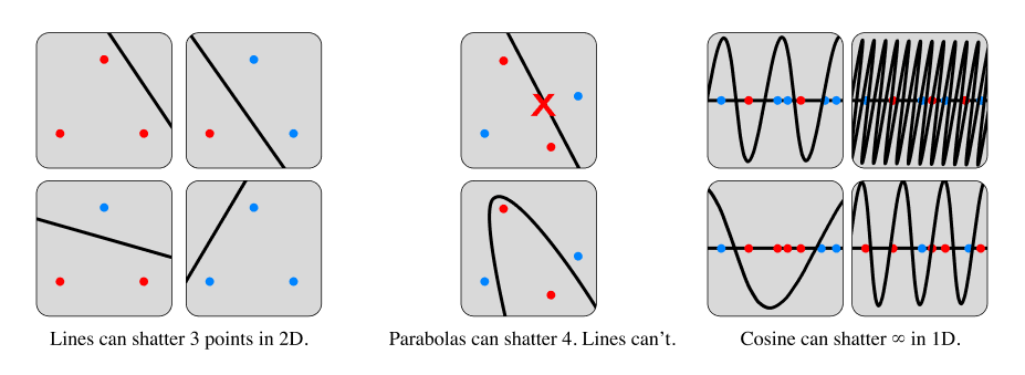
We start by defining the growth function, which is the maximum number of different ways a model class can classify an arbitrary set of inputs $(x_1,\dots ,x_m)\in X^m$:

$$g_F\left(m\right):=\underset{(x_1,\dots ,x_m)\in X^m}{max}\left|\right\{(f_w\left(x_1\right),\dots ,f_w\left(x_m\right)):w\in W\left\}\right|\le 2^m.$$

If the growth function saturates its upper bound, then we say that the model class "shatters" that set of samples. This means the model class always contains a model that can perfectly classify the given inputs under any possible relabeling.

So a straight line can shatter a set of three non-collinear points on a 2D, but not four. A parabola can shatter four points but not five. And so on.

Then, the VC dimension is the largest set of points that can be shattered by a given model class.

$$d_{VC}:=max\{m\in N:g_F(m)=2^m\}$$

In terms of the VC dimension $d_{VC}$ we end up satisfying the PAC bound if our sample size is

$$n\ge \frac{c}{ϵ}(d_{VC}\log \frac{1}{ϵ}+\log \frac{1}{\delta }),$$

where $c$ is a constant. We replaced the term depending on the size of $F$ in the original PAC bound with a term that depends on the VC dimension of a potentially infinite model class.

The VC dimension is straightforward to generalize to more realistic settings (e.g., the Natarajan dimension for multi-class classification and Pollard's pseudo-dimension for regression). It's also possible to derive tighter bounds by including information about the shape of the data distribution as in the fat-shattering dimension.

The problem with applying these variants to neural networks is that we are typically working in or near the over-parametrized regime, where the number of parameters is larger than the number of samples. In this regime, as Zhang et al. showed, we can typically shatter the entire training set, so $d_{VC}$ is on the order of $n$ and the bound is not satisfied for reasonable tolerances.^[5] 

Rademacher complexity

The basic idea behind the Rademacher complexity, like the VC dimension, is to measure how well a function class can fit random noise. First, let us define the empirical Rademacher complexity of a model class $W$ with respect to a dataset $D_n$:

$${\mathrm{Rad}}_{D_n}\left(W\right):=E_{p\left({\sigma }_1\dots {\sigma }_n\right)}\left[\underset{w\in W}{sup}\frac{1}{n}\sum _{i=1}^n{\sigma }_i{f}_w\right(x_i\left)\right].$$

The idea is to choose a set of random Rademacher variables, $\{{\sigma }_i{\}}_{i=1}^m$ that take on the values $-1$ and $1$ with equal probability. We apply these random sign flips to each of our individual predictions and take the average. Then, we maximize the average flipped prediction over models. Finally, we average over different sign flips.

Intuitively, imagine separating your dataset into a train and test set. The Rademacher complexity measures the maximum discrepancy over the model class between your predictions for the two sets.

From this, the Rademacher complexity of $W$ with respect to a probability distribution, $q\left(D_n\right)$ is the expectation of the empirical Rademacher complexity taken over draws of the dataset:

$${\mathrm{Rad}}_n\left(W\right):=E_{q\left(D_n\right)}\left[{\mathrm{Rad}}_{D_n}\right(W\left)\right].$$

In terms of the Rademacher complexity, we obtain the PAC bound when

$$ϵ\le 2{\mathrm{Rad}}_n\left(W\right)+3c\sqrt{\frac{\log \left(2/\delta \right)}{2n}},$$

where $c$ is a constant that depends on the range of functions in $F$.

Since the Rademacher complexity is uniform across $W$, it runs into the same issues as the VC dimension. Another problem is that it is not necessarily easy to calculate. In practice, learning theorists often resort to further upper-bounding the Rademacher complexity in terms of covering numbers.

Covering numbers

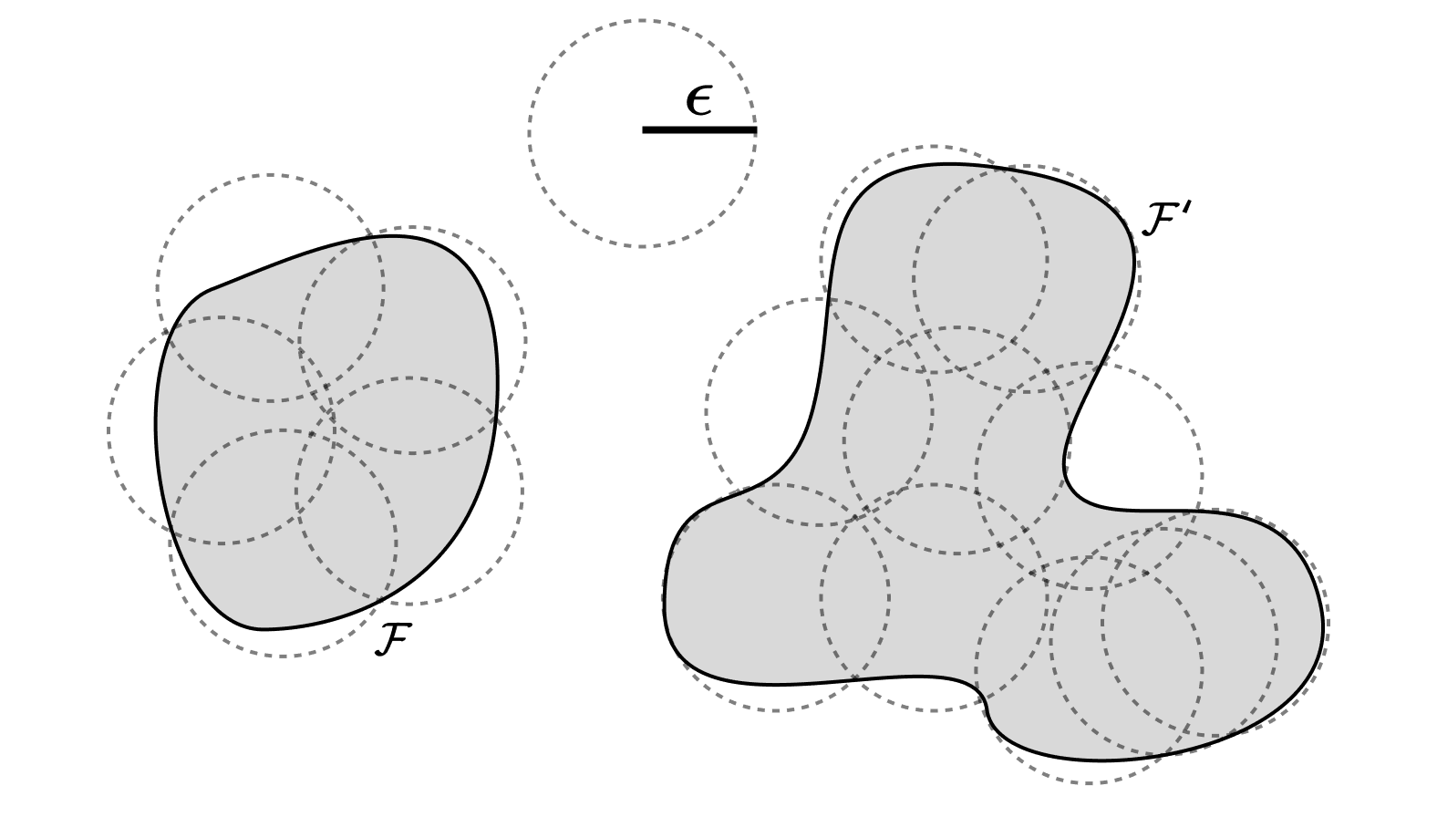
The covering number is the number of spherical balls of a given size needed to cover a given space (with overlaps allowed). The idea is that we're "coarse-graining" the model class with a finite collection of representative elements.

In terms of $N_r\left(W\right)$, the covering number of $W$ for balls of radius $r=ϵ/2c$, we satisfy the PAC bound if

$$n\ge \frac{2c}{{ϵ}^2}\left(\log 2N_r\right(W)+\log \frac{1}{\delta }),$$

where $c$ is some constant. 

By default, $N_r\left(W\right)$ will scale exponentially with model dimension $d$, so the resulting bounds don't become much tighter than VC. However, conceptually, this is getting closer at the idea of model-subclass complexity. The differences are that covering numbers still treat each subclass as identical, and we're not yet coarse-graining in any principled way. 

Single-model complexity

Instead of constraining entire model classes, it's much more tractable to study the complexity of individual models. Most notions of single-model complexity are based on the idea of complexity as sensitivity to noise: noise applied to the inputs (margin theory), noise applied to the weights (minimum sharpness/flatness), and noise applied to the training samples (algorithmic stability & robustness).

Margins

Margin theory studies the eponymous margin, which is the minimum distance from a sample to the decision boundary of a classifier. The larger the margin, the more robust the classifier is to small perturbations in the input data, thus the better we expect it to generalize to novel data.

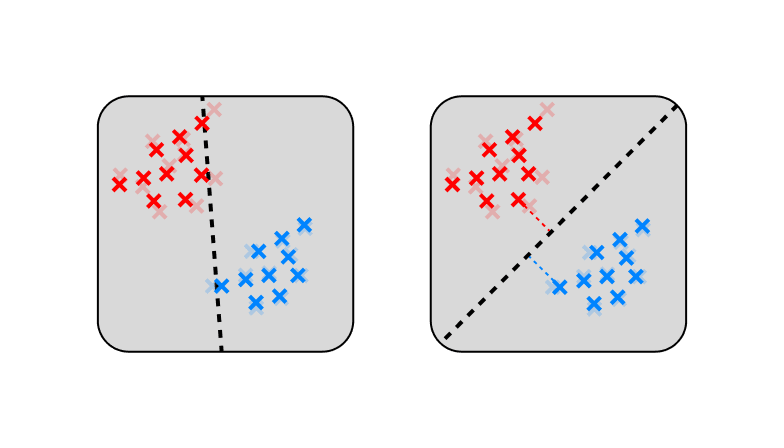
This dates back to the good old days of support vector machines (SVMs) for which you can explicitly calculate margins and use them to design more robust classifiers (see Vapnik (1995)) . With DNNs, calculating margins is intractable.

The more fundamental problem is that the assumption that "large margins = better generalization" doesn't hold for realistic models. Which of the following two decision boundaries would you say generalizes better?

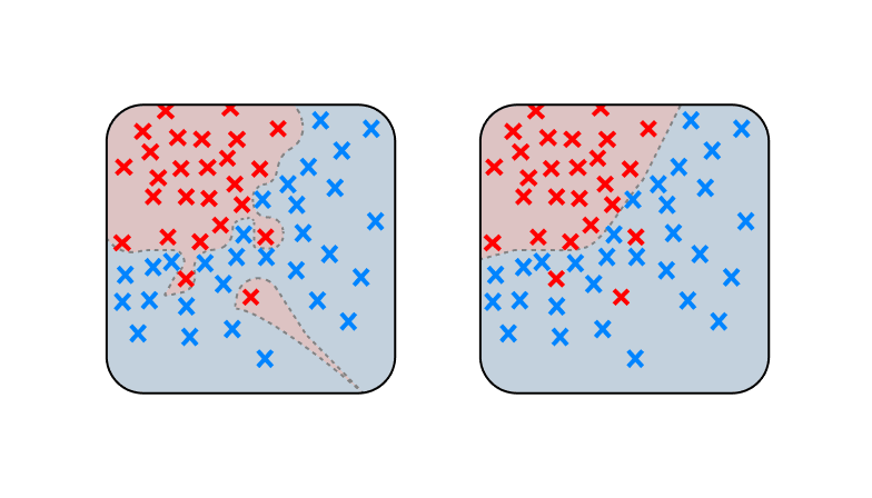
Margin theory certainly seems to have some explanatory power, especially in settings with simpler and more structured data (e.g., Mohamadi et al.  2023). The basic idea of studying sensitivity to input noise remains a good one. It's just that the specific focus on margins appears to be overemphasized.

Minimum flatness/sharpness

Where margin theory hinges on the intuition that robustness to input perturbations should lead to generalization, "minimum flatness" hinges on the intuition that robustness to weight perturbations should lead to generalization.

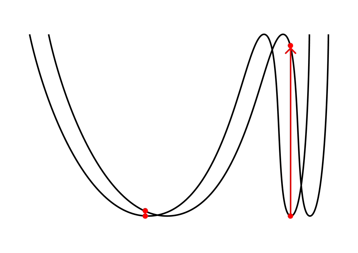
If the curvature (as measured by the Hessian) of the loss landscape is low, then a small change to the weights will mean a small change in the loss. So we might expect the loss landscape shouldn't change much if we perturb it by introducing novel samples (=ask it to generalize). Conversely, if the curvature is high, the model is more complex and likely to generalize poorly.

As is true for all many ideas in deep learning, this dates back to a paper by Hochreiter and Schmidhuber written in the 90's. They offer intuition built on the minimum description length (MDL) principle from algorithmic complexity theory. In the language of MDL, fewer bits are needed to specify the location of "flat" minima, and simpler functions should generalize better.

Keskar et al. (2017) demonstrate that minibatch SGD converges to flatter minima and that this correlates strongly with the generalization error. However, Neyshabur et al. (2017a) and Dinh et al. (2017) point out that this naive approach is flawed: sharpness can be arbitrarily scaled by reparametrizations, and models trained on random labels routinely have flatter minima than models trained on true labels. To remedy this, Kwon et al. (2021) propose adaptive sharpness, which is invariant to reparametrizations and seems to correlate well with generalization error.

As it turns out, adaptive sharpness isn't enough to save sharpness theory. Andriushchenko et al. (2023) find that counter to classical intuitions, sharpness — and even the smarter reparametrization-invariant notions — correlate poorly or even negatively with generalization in transformers on larger datasets. In their words, "sharpness is not a good indicator of generalization in the modern setting."

There's a more fundamental problem: neural networks are singular, so modeling the loss landscapes locally with paraboloids is invalid [LW · GW]. Studying sensitivity to changes in weights requires more advanced tooling from algebraic geometry.

Algorithmic stability and robustness

Yet another notion of sensitivity to noise is sensitivity of the final model to changes in the training set. This is the idea behind Bousquet and Elisseeff's (2000) algorithmic stability: if changing a training sample doesn't change a model's performance, the empirical risk should have low variance.

A learning algorithm is said to have uniform stability $\beta$ if

$$\underset{i}{max}\left\{|\ell \left(f_{w\left(D_n\right)}\right(x_i),y_i)-\ell \left(f_{w\left(D_n^{\setminus i}\right)}\right(x_i),y_i)|\right\}\le \beta .$$

It's an upper bound to how much the loss changes on any one sample $(x_i,y_i)$ in the training set upon omitting that sample during training.

This leads to the following PAC-style bound for the specific weights obtained by the learning algorithm (Bousquet and Elisseef 2002):

$$G_n\left(f_w\right)\le 2\beta +(4n\beta +1)\sqrt{\frac{\log \frac{1}{\delta }}{2n}}.$$

This avenue of research has strong parallels to work on influence functions (e.g., Grosse et al. 2023) and to work on differential privacy starting with Dwork et al. (2006), which is about making sure that you can't tell whether a sample belongs to the training set. It's also been extended to algorithmic robustness by Xu and Mannor (2012), which looks at sensitivity to changing the entire dataset rather than individual examples.

This is getting closer to the perspective we already glimpsed with the PAC-Bayes data-dependent priors, where model complexity was related to how the model changes in response to additional data. It's a perspective we'll see again in SLT.

Model-subclass complexity

So far, we've seen generalization as a question about expressivity of a model class (how well it can fit random noise), and we've seen generalization as a question about robustness of specific models (how well they can "resist" small amounts of noise). Another possibility is to view generalization as a question about the robustness of the distribution of learned models $p\left(w|D_n\right)$. 

In this section, we'll explore a variety of complexity measures that involve examining how a distribution of learning machines changes, particularly in response to new data. We'll see in the next section that this turns studying generalization into a problem of comparing subclasses of weights. 

Information-theoretic metrics

One of the more principled approaches to studying generalization in modern deep learning theory comes from a strand of information-theoretic complexity measures that developed in parallel to (and in isolation from) modern PAC-Bayes theory. The complexity measures that show up in these bounds are information-theoretic metrics in terms of the various distributions over weights and data. The associated bounds are in expectation over weights — not uniform.

We already saw one example in terms of the mutual information between weights and data, $I(w\parallel D_n)$, which is the Kullback-Leibler divergence between the joint distribution and the product of the marginal distributions,

$$I(w\parallel D_n)=D_{KL}\left(p\right(w,D_n)\parallel p(w\left)q\right(D_n\left)\right).$$

This may be the most intuitive notion of complexity so far: models are more complex if they contain more information about the dataset.

We saw another example in the KL divergence between the posterior and prior $D_{KL}(p\parallel \phi )$ that showed up in the PAC-Bayes example. Models are "simpler" if their weights are "closer" to their initial values.

Many of the bounds involving these KL divergences can be generalized in terms of other divergences, such as the broader family of f-divergences, Rényi divergences, (conditional) maximal leakages, Wasserstein metrics, etc. There are many more tricks to squeeze out a few extra bits of generalization here and there.

Unfortunately, these bounds run into problems when applying them to real-world systems because these information-theoretic metrics are typically intractable to calculate or even estimate. 

Compressibility

Compression-based bounds build on the same idea behind minimum flatness/sharpness of robustness to changes in weights. If the model is highly compressible and you can discard many weights without impacting performance, the model's effective dimensionality is lower than its apparent dimensionality. It's simpler than it looks and should therefore generalize.

Arora et al. (2018) provide the seminal treatment. They convert a given model into a set of simpler, compressed models, which lets them apply the tooling of the typical model-class-complexity bounds to this family. The framework doesn't directly predict the generalization of the original model but of the constructed subclass. 

Zhou et al. (2019) combine this idea with the idea of data-dependent priors that shows up in PAC-Bayes theory. The posterior is chosen to be a Gaussian centered at the learned weights and the prior is chosen to be the set of compressed weights (obtained by pruning). Similar to the approach taken by Dziugaite and Roy (2017), they add in a dash of minimum sharpness by overlaying Gaussian noise over the non-zero weights. The resulting bounds are among the first to be non-vacuous for neural networks, but they're still far from tight. 

The main limitation of this approach seems to be that these subclasses are currently constructed in a rather ad-hoc way. For example, singular posteriors are not asymptotically Gaussian, so modeling posteriors as Gaussian is unfounded. In addition, neural networks have many more kinds of degeneracy than just weights that can be pruned (see for example Hanin and Rolnick 2019). What this means is that current bounds likely severely underestimate how compressible neural networks really are. 

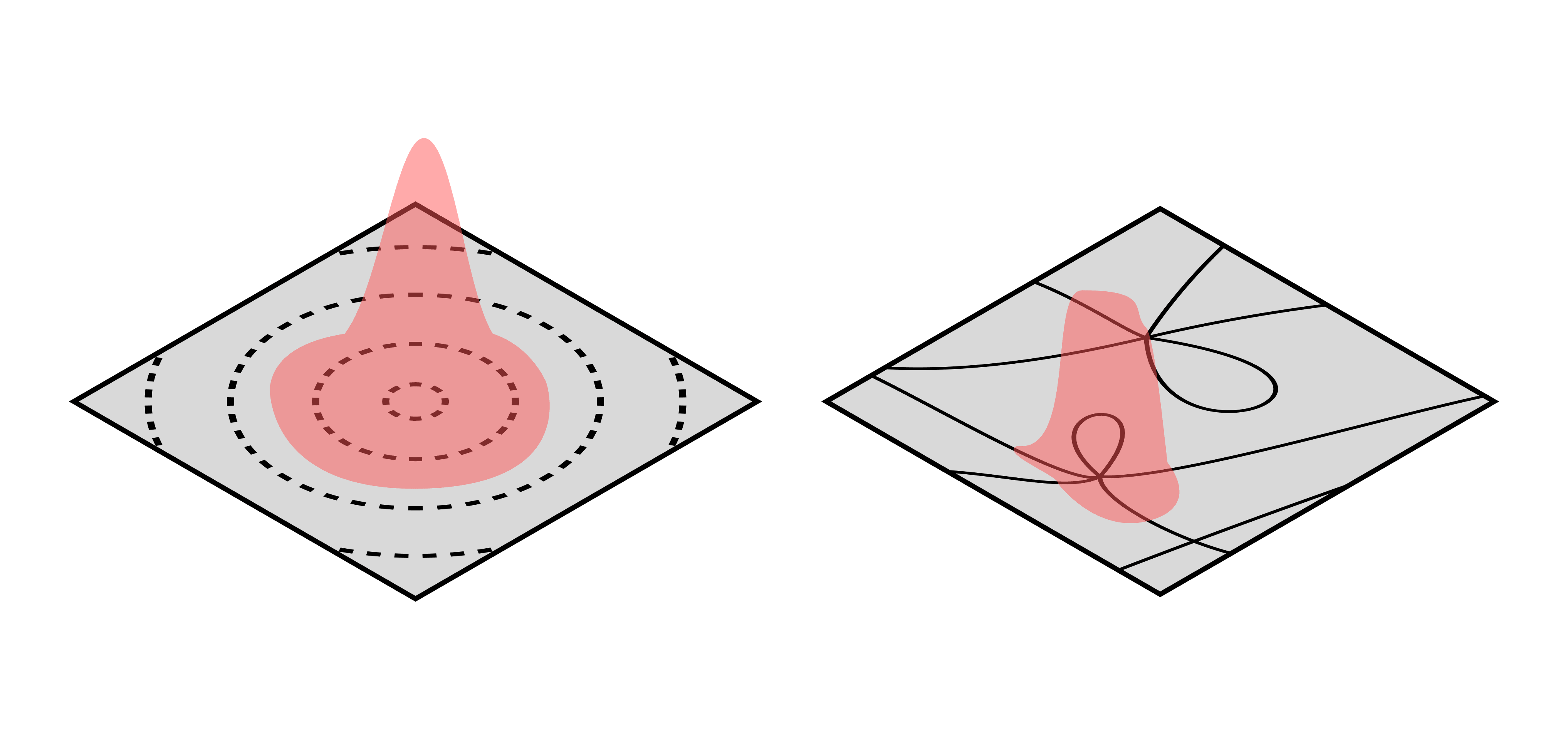
One contender for a more natural notion of compressibility is SLT's learning coefficient. Though the exact link with ideas such as the Minimum Description Length (MDL) principle and compressibility is an open question, it's clear that the learning coefficient captures a much richer set of degeneracies that, for example, the number of weights you can prune. 

The free energy / stochastic complexity

Given a likelihood and prior, we can define the Bayesian free energy (or stochastic complexity) $F_n$ as the negative logarithm of the marginal likelihood (or model evidence):

$$\begin{array}{cc}{F}_n& =-\log p\left(D_n\right),\\ & =-\log {\int }_{W}p\left(w|D_n\right)\phi \left(w\right)dw,\\ & =-\log {\int }_w{e}^{-n{L}_n\left(w\right)}\phi \left(w\right)dw,\end{array}$$

where $L_n\left(w\right)=-\log p\left(w|D_n\right)$ is the negative log likelihood. 

The most important result of SLT (Watanabe 2009) is the asymptotic form of the free energy as $n\to \infty$:

$$F_n=n{L}_n\left(w^{\ast }\right)+\lambda \log n-(m-1)\log \log n+F^R\left(\xi \right)+o_p\left(1\right).$$

From the perspective of complexity, we're more interested in the normalized free energy, 

$$F_n^0=F_n-n{L}_n\left(w^{\ast }\right)=\lambda \log n-(m-1)\log \log n+F^R\left(\xi \right)+o_p\left(1\right).$$

The important feature of this composite notion of complexity is that this expression involves the number of samples $n$. Seeing more data makes you more certain about the function you're trying to learn and so warrants learning more complex fits. This means we want a notion of complexity that is defined relative to the amount of data we've seen. 

In the rest of this section, we'll examine each of the terms in this expression individually. Afterwards, we'll see how this formula leads to viewing generalization in terms of subclasses. 

Learning coefficient

As I've argued before [LW · GW], the learning coefficient is the "correct" notion of model complexity (at least in the Bayesian setting).

Here's what we currently know:

• The learning coefficient is the second-leading term in the free energy formula, 

$$F_n=n{L}_n\left(w^{\ast }\right)+\lambda \log n-(m-1)\log \log n+F^R\left(\xi \right)+o_p\left(1\right).$$

• The learning coefficient is (half) the "effective dimension" that controls how weight space volume scales scales as you approach the bottom of the loss landscape (similar to the Minkowski dimension).
• If your loss landscape is real analytic (which is the case for many realistic models), then the learning coefficient is the maximal real log canonical threshold (RLCT) of that function's vanishing set. This is a geometric quantity that measures how "complex" the model's most "complex" minimum-loss singularity is.
• Up to highest order, the "per-sample" learning coefficient is equal to the increase in the expected normalized free energy,  where $F_n^0:=F_n-n{L}_n\left(w^{\ast }\right)$:

$$\frac{\lambda }{n}\approx E_{q\left(D_{n+1}\right)}\left[F_{n+1}^0\right]-E_{q\left(D_n\right)}\left[F_n^0\right].$$

• Physically, the learning coefficient is the first term in the expansion of the heat capacity, which measures how much a system's temperature changes in response to heat flowing in or out of the system. Heuristically, the learning coefficient tells us something like how expensive it is to change the loss, 

$$\lambda =-n^2{E}_{q\left(D_n\right)}\left[\frac{{\partial }^2{F}_n}{\partial n^2}\right].$$

• The learning coefficient is the leading term for the asymptotic expected Bayes generalization error. For the expected Gibbs generalization error, it is leading order alongside a related invariant known as the singular fluctuation $\nu$:^[6] 

$$\begin{array}{cc}{E}_{q\left(D_n\right)}\left[G_n^B\right]& \to L\left(w^{\ast }\right)+\frac{\lambda }{n},\\ E_{q\left(D_n\right)}\left[G_n^G\right]& \to L\left(w^{\ast }\right)+\frac{\lambda +\nu }{n}.\end{array}$$

Note that these last asymptotes are tight equalities on both sides. That's a lot more than other complexity measures can say. 

Singular fluctuation

The singular fluctuation $\nu$ that shows up in the Gibbs generalization error is a more mysterious quantity. Asymptotically, it is:

$$\nu \to \frac{E_{q\left(D_n\right)}\left[V_n\right]}{2},$$

where $V_n$ is the empirical variance,

$$V_n=\sum _{i=1}^n\left\{E_{p\left(w|D_n\right)}\right[\left(\log p\right(y_i|x_i,w\left){)}^2\right]-E_{p\left(w|D_n\right)}\left[\log p\right(y_i|x_i,w\left){]}^2\right\}.$$

The singular fluctuation measures the average scalar curvature of the free energy with respect to sample strength. To see this, let us express the negative log likelihood as

$$n{L}_n\left(w\right):=-\sum _{i=1}^n\log p(y_i|x_i,w)=:\sum _{i=1}^n{\ell }_i\left(w\right),$$

and couple the negative log sample likelihoods to a sample-dependent inverse temperature $\overrightarrow{\beta }$. This allows us to vary the relative importance of different samples:

$$p^{\overrightarrow{\beta }}\left(w|D_n\right)=e^{-\overrightarrow{\beta }\cdot \overrightarrow{\ell }\left(w\right)}.$$

Then, we can express

$$V_n={\mathrm{Tr}\frac{{\partial }^2{F}_n^{\overrightarrow{\beta }}}{\partial {\beta }_i\partial {\beta }_j}|}_{{\beta }_i={\beta }_j=1},$$

and thus

$$\nu =\frac{1}{2}{E}_{q\left(D_n\right)}{\left[\mathrm{Tr}\frac{{\partial }^2{F}_n^{\overrightarrow{\beta }}}{\partial {\beta }_i\partial {\beta }_j}\right]}_{{\beta }_i={\beta }_j=1},$$

Beyond this, not much is currently known about the singular fluctuation and what it means for real-world systems. 

Multiplicity

After the learning coefficient, the multiplicity $m$ controls the next-leading term ($\log \log n$) in the free energy formula and in the two generalization errors. So it influences generalization but less than the learning coefficient.

Like the singular fluctuation, little is known about its role in real-world systems, and it doesn't have an easy-to-understand meaning. This is different from the standard "multiplicity" of algebraic geometry; the SLT multiplicity is a subtle invariant associated to the RLCT.  

Weight norm

The weight norm is probably the most obvious alternative to explicit parameter count as a measure of model complexity. It's common knowledge that regularization terms like weight decay encourage simpler models that generalize better. Naturally, learning theorists have worked hard to obtain bounds that involve regularization strengths and weight norms (see, for example, Neyshabur et al. 2015, Golowich et al. 2019).

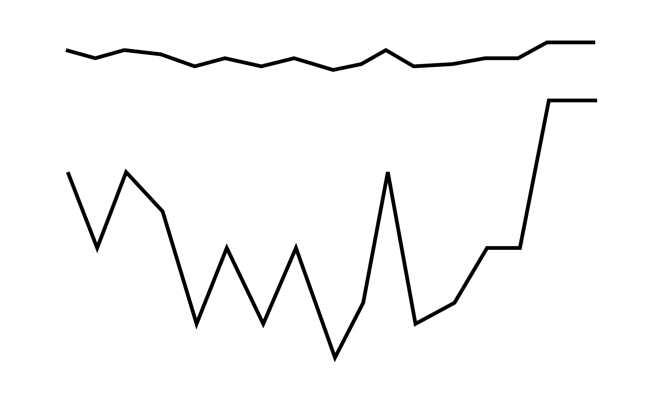
Unfortunately Zhang et al. also thought to test whether neural networks can fit random noise in the presence of regularization. They can, which means that weight norm alone is not enough to explain observed generalization performance. Incorporating weight norms might lead to tighter bounds, but these are marginal improvements and not enough to resolve the mystery.

Formally, this is because the weight norm is a lower order contribution to the free energy than the learning coefficient and multiplicity. After the multiplicity term, there's a stochastic term $F^R\left(\xi \right)$ related to randomness in draws of the dataset and a constant order term $o_p\left(1\right)$ which contains the contribution of the prior. With a standard choice of Gaussian prior, this is where the weight norm would show up. So the weight norm has influence on behavior and generalization, but less than you might expect in a Bayesian setting.

Thermodynamics of generalization

Internal model selection

In what sense does this last set of complexity measures relate to model subclasses? 

To reveal the link, let us coarse-grain the weight space into a collection of compact subsets $W_{\alpha }$ that cover $W$. For now, the particular choice of partitioning is arbitrary (up to a few technical conditions). This allows us to re-express the free energy $F_n$ as a combination over the local free energies $F_n\left(W_{\alpha }\right)$ of each subclass (with an adjusted prior ${\phi }_{\alpha }$ and restricted domain of integration):

$$\begin{array}{cc}{F}_n& =-\log \sum _{\alpha }{\int }_{W_{\alpha }}p\left(D_n|w\right){\phi }_{\alpha }\left(w\right),dw,\\ & =-\log \sum _{\alpha }{e}^{-F_n\left(W_{\alpha }\right)}\\ & \approx \underset{\alpha }{min}{F}_n\left(W_{\alpha }\right).\end{array}$$

The last step follows from the log-sum-exp approximation, which is how nature implements the minimum/maximum function. 

A classic result by  I.J. Good is that choosing the optimal model class (a problem known as model selection) is equivalent to choosing the model class that minimizes the free energy. What the above formula then tells us is that, for any arbitrary choice of coarse-graining, learning machines automatically perform internal model selection, where they minimize the local free energy and thereby choose the optimal model subclass. 

Why model subclasses

It's straightforward to turn global expressivity measures like the VC dimension into model-class expressivity measures simply by restricting their domain. Similarly, it's possible to reinterpret local robustness measures like algorithmic stability in a probabilistic setting as observables associated to a subclass of weights. These approaches are still meaningfully different from the sense in which SLT observables are associated to model subclasses.  

To see this, we combine the perspective of internal model selection with the free energy formula. There is an analogous form of this formula for the local free energy: 

$$\begin{array}{cc}{F}_n\left(W_{\alpha }\right)& =-\log {\int }_{W_{\alpha }}p\left(D_n|w\right){\phi }_{\alpha }\left(w\right)dw,\\ & =n{L}_n\left(w_{\alpha }^{\ast }\right)+{\lambda }_{\alpha }\log n+(m_{\alpha }-1)\log \log n+F^R\left(\xi \right)+o_p\left(1\right),\end{array}$$

where now $w_{\alpha }^{\ast }$ is a minimizer of $L_n$ within $W_{\alpha }$, and ${\lambda }_{\alpha }$ is the maximum local RLCT associated to the set of minima with associated multiplicity $m_{\alpha }$.

Even though the free energy (local or global) is associated to a dense region of weight space, its limiting form is dominated by a very special measure-zero subset of weights within those regions — not just the set of minima within $W_{\alpha }$ but the set of the most singular points within those minima. Whatever coarse-graining $W_{\alpha }$ you choose, the performance of subclasses and the selection process between them will be dominated by the values of a principled set of observables associated to these singularities: the learning coefficient, singular fluctuation, and multiplicity. 

Not only do SLT observables emerge more naturally from the theory, but they're inherently non-local. Given a model at an arbitrary choice of weights, as you continue to draw more samples, the changes in the probability density at that point will be dominated by the set of nearby singularities. So you can't understand generalization purely in terms of the behavior of an individual weights. Likewise, you can't understand generalization purely in global terms. Depending on the "timescale" involved (the number of samples you've drawn), different singularities will dominate the learning process and thus generalization. Subclasses are the natural unit to study. 

Why neural networks generalize

For regular models, the learning coefficient and multiplicity are constant, so the process of internal model selection typically reduces to simply finding the subclass that minimizes loss. For singular models, the process is very different: the learning coefficient and multiplicity can vary, so minimizing the free energy involves trading off accuracy against complexity that depends on the current number of samples.  

Let's focus on just the first two terms:

$$F_n\left(W_{\alpha }\right)\approx n{L}_n\left(w_{\alpha }^{\ast }\right)+{\lambda }_{\alpha }\log n.$$

To minimize this formula over different submodels for a given $n$, you can either lower the loss $L_n$ or the complexity ${\lambda }_{\alpha }$. This is yet another incarnation of the Occam's razor tradeoff between accuracy and complexity. Unlike the other incarnations, internal model selection means singular Bayesian learners perform this tradeoff automatically.

What happens as you change $n$? As $n$ increases, the trade-off between accuracy and complexity will increasingly favor the linear accuracy term over the logarithmic complexity term. So models will become more accurate at the cost of additional complexity — a cost warranted by the additional information gained from seeing more samples. This lets singular models maintain the optimal trade-off between memorization and generalization throughout the entire learning process.

This automatic trade-off explains why singular learning machines like neural networks are able to generalize in practice. But it doesn't explain the related question of why the set of low-loss solutions should contain any points with low RLCT. As discussed in the previous post [LW · GW], this seems to require a deeper understanding of what kinds of data are "natural" and what is special about neural network's architectures. Some mystery remains. 

How neural networks generalize

We're not just interested in why learning machines can generalize. We're interested in how. What are the particular generalization strategies a neural network will adopt?

There's been plenty of work investigating the "inductive biases" of neural networks, but this literature is still in an early stage. The results are highly empirical and lack the kind of unified mathematical formalism underlying the study of generalization bounds.^[7] Can we do better? What is the right mathematical formalism for studying the inductive biases of learning machines?

SLT offers a few hints. The learning coefficient tells us of a deep link between generalization and changes in the posterior/free energy. This puts generalization and optimization on the same footing, and it's a link we saw pop up in a few other places: data-dependent priors (where the bound involves the number of bits between learning machines under different selections of data), algorithmic stability/robustness (where the bound is in terms of how much a model changes in response to additional samples), and the bounds involving the mutual information between weights and data.

In particular, SLT tells of a link between generalization and geometry, particularly changes in geometry. This geometry follows from the data-generating process and the symmetries of your model class. In hindsight, it's not surprising that such a link exists. The idea that symmetries determine physical properties is foundational to modern theoretical physics. Why would learning machines be the exception?

From this perspective, the natural question to ask is how much more information we can extract from local geometry. Can we use geometry to learn something about neural networks' internal structure? In particular, when physicists talk about structure, they mean correlation functions — in learning theory, this would mean tensors like $E\left[w_i{w}_j\right]$ and $E\left[w_i{w}_j{w}_k\right]$. Algebraic geometry and statistical physics have highly sophisticated tools for studying this finer-scale geometric structure — tools that, until now, have been neglected by learning theory.

As soon as we start studying correlation functions, we move past the domain of scalar thermodynamics to the realm of statistical physics. So maybe what's needed to move from why generalization to how generalization is a corresponding change in our perspective of learning: from a thermodynamics of learning to a statistical physics of learning.

Future research

There is lots of low-hanging fruit in terms of introducing the broader field of generalization theory to singular learning theory. There's the grunt work of contorting SLT's results into more typical (PAC-Bayes) kinds of bounds and showing that you can beat the current state-of-the-art generalization bounds. There's fleshing out the connections to compression theory, algorithmic stability, and margin theory (e.g., uniform stability looks very similar to the singular fluctuation). There's more interesting work in bridging SLT to the information-theoretic generalization theory, which might yield new perspectives on ideas in SLT (e.g., an MDL-grounded framing of SLT). 

At Timaeus [LW · GW], we're currently focused on importing the tooling of statistical physics into learning theory to investigate structure from a geometric perspective. The first time around, it took decades and hundreds of physicists to establish statistical physics. We're optimistic we can do it faster this time, but we will need help. If any of this interests you, please reach out. 

Thank you to @Daniel Murfet [LW · GW], @Edmund Lau [LW · GW], @Zach Furman [LW · GW], @Liam Carroll [LW · GW], @Stan van Wingerden [LW · GW], Simon Pepin Lehalleur, and @Alexander Gietelink Oldenziel [LW · GW] for feedback on this post.

If you want to learn more about generalization theory, check out Hellström et al. (2023). 

1. ^{^}

   I'll be focusing on the supervised setting where we're mapping inputs $x_i$ to outputs ${\hat{y}}_i=f_w\left(x_i\right)$ using a parametrized, deterministic function $f_w$. The discussion transfers straightforwardly to other settings such as density estimation.

2. ^{^}

   Sorry for perpetuating more varieties of terrible notation for expectation operators.

3. ^{^}

   The link is that you recover Bayes rule if apply the MaxEnt principle to empirical risk minimization. In this approach, Bayes rule is called the Gibbs distribution.

4. ^{^}

   For the details, I'll recommend Hellström et al. (2023). At a high-level, there are typically two steps involved. First, you do a change of measure from the probability distributions you're given to another probability distribution that's easier to handle. This conversion comes at the cost of introducing a penalty term. Second, you apply one or more concentration inequalities.

5. ^{^}

   This isn't even a particularly novel problem with the VC dimension. For many model classes of practical interest (e.g., the sinusoid depicted in the figure on the right hand side), the VC dimension is infinite, so we're back at the starting block. 

6. ^{^}

   The similarity with the preceding bullet follows from the fact that the free energy or "stochastic complexity" is a moment-generating functional. We can generate expectation values of arbitrary observables by taking derivatives (or finite differences when $n$ is integer).

7. ^{^}

   Okay maybe this is a bit of an exaggeration.

9 comments

Comments sorted by top scores.