A comparison of causal scrubbing, causal abstractions, and related methods

post by Erik Jenner (ejenner), Adrià Garriga-alonso (rhaps0dy), Egor Zverev · 2023-06-08T23:40:34.475Z · LW · GW · 3 comments

Contents

  Introduction
  Use cases for definitions of explanations
  Setup
  Overview of different methods
    Causal abstractions
    Interchange interventions/Resampling ablations
    The Geiger et al. algorithm
    Causal scrubbing
    Locally consistent abstractions
  Axes of differences between methods
    Set of accepted explanations
    Checking consistency for intermediate nodes vs output only
    Explicit vs implicit τ-maps
    Global vs local consistency and activation distributions
    Only allowing interventions that leave H unchanged
    Expectations vs sample-wise errors
    Treeification
    Computational complexity
    Compounding errors and chaotic computations
    Multiple simultaneous interventions
  Discussion
    A common framework
    Combining components in different ways
    How strict do we want our criterion to be?
    Different conceptual goals
  Conclusion
  Appendix
None
3 comments

Summary: We explain the similarities and differences between three recent approaches to testing interpretability hypotheses: causal scrubbing [LW · GW], Geiger et al.'s causal abstraction-based method, and locally consistent abstractions [AF · GW]. In particular, we show that all of these methods accept some hypotheses rejected by some of the others.

Acknowledgements: Thanks to Dylan Xu and Joyee Chen for many conversations related to this post while they were working on their SPAR project! And thanks to Atticus Geiger, Nora Belrose, and Lawrence Chan for discussions and feedback!

Introduction

An important question for mechanistic interpretability (and other topics) is: what type of thing is a mechanistic explanation of a certain neural network behavior? And what does it mean for such an explanation to be correct?

Recently, several strands of work have (mostly independently) developed similar answers:

• Atticus Geiger and his collaborators at Stanford have been publishing on applying causal abstractions to neural networks since 2020. They interpret both neural networks and potential explanations as causal models and say that an explanation is correct if it is a valid causal abstraction. To test an explanation empirically, they developed interchange interventions, which perform the same interventions on the neural network’s activations and on the explanation, after which they check that the outputs after intervention are the same.
• Redwood Research has been using the Causal Scrubbing [LW · GW] algorithm to test interpretability hypotheses. Again, computational graphs are used as explanations, and the validity of an explanation is checked by performing interventions (or ablations) on activations.
• I (Erik) have written about a framework for abstractions of computations [AF · GW] that is very similar to causal abstractions (and many other related ideas, like abstract interpretation or bisimulation). We will call the particular definition of abstractions given in that post locally consistent abstractions (LCAs).

In this post, we explain these different approaches and highlight their similarities and differences. We also give examples of "disagreements" where some approaches accept an explanation and others reject it, and we discuss some conceptual takeaways.

This post is meant to be self-contained and doesn't require familiarity with any of the work we are discussing. (In fact, it may be a good first introduction to all these methods.)

The approaches we listed certainly aren’t the only possible definitions of “explanations”, for example heuristic arguments could provide a rather different notion. There is also much older work with similar ideas. We focus on these because

1. They are particularly similar to each other (unlike heuristic arguments).
2. They are all pursued by people specifically interested in neural networks, interpretability, or AI safety (unlike earlier work on abstraction in causality or theoretical CS).

Use cases for definitions of explanations

Historically, the approaches we’ll discuss have been used for different purposes (for example, causal scrubbing has mostly been used to check interpretability hypotheses, whereas Geiger et al. have also been working on interchange intervention training, allowing them to enforce certain structures onto neural networks).

But this is mostly historical accident, so we want to clarify that these methods (and many others) can all be used for several different purposes:

• Conceptually clarifying what an “explanation” is or should be. Trying to formalize the concept can reveal important subquestions.
• Testing interpretability hypotheses in a principled way (and giving a general format for formally describing hypotheses).
• Automatically searching for explanations: you need to define what "explanations" are (to have a search space) and what makes an explanation correct.
• Enforcing certain (interpretable) structures on networks: in this case, the explanation is fixed, while the network is optimized to fit the explanation (and do well at some task).
• Mechanistic anomaly detection [AF · GW]: you can learn an explanation of a given model on a reference distribution of “normal” inputs and then check whether the explanation is still correct on some new input. (This requires being able to judge correctness on individual inputs, but all three methods here can do that.)

Setup

Throughout this post, we will use the Causal Scrubbing [LW · GW] setup (with notation similar to Geiger et al. (2023)):

• There is a low-level computation described by a (static and deterministic) computational graph $L$. In practice, this could be a graph description of a particular neural network. Equivalently, you can think of $L$ as an (acyclic) deterministic causal model.
• We have a distribution $D$ of inputs, and we want to explain the behavior of $L$ on $D$.
• An explanation is a high-level computational graph $H$, together with an injective graph homomorphism $\Pi :H\to L$ on nodes.^[1] $\Pi$ describes which node in $H$ is supposed to correspond to which node in $L$. We'll write inputs to $\Pi$ as subscripts, ${\Pi }_X:=\Pi \left(X\right)$ for a node $X\in H$. $H$ typically needs to have the same input and output types as $L$ (with causal scrubbing being an exception, as we'll see).

In this setting, all three methods define what it means for $(H,\Pi )$ to be a correct explanation, as well as graded notions that can quantify “how incorrect” $H$ is. (We will often just refer to the explanation as $H$, even though $\Pi$ is also part of it.)

Some notes on this:

• The setting is the same as in the causal scrubbing post [LW · GW], we just follow the causal abstraction notation instead. $L$ corresponds to $G$ in the causal scrubbing post, $H$ to $I$, and $\Pi$ to $c$.
• Causal abstractions are formulated more generally, where a single node in $H$ can correspond to multiple nodes in $L$ (so ${\Pi }_X$ is a set of nodes in $L$). They also don't require $\Pi$ to be a homomorphism. Locally consistent abstractions were originally formulated even more generally, for computations other than static graphs (e.g. Turing machines). But even the simple setting we use in this post leads to many interesting differences between methods.
• We need some way of turning a neural network into a graph $L$, i.e. we need to decide what the individual nodes should be. We won’t discuss that problem in this post since it is orthogonal to the main algorithms we're comparing.
• If we only want to explain some aspect of the output (i.e. up to an equivalence relation), we make that choice part of $L$ by adding a final node at the end that “forgets” all the information we don’t want to explain. For example, causal scrubbing is usually applied to explanations of the loss instead of the full output of the network. Similarly, if the explanation $H$ only takes in part of the input, we implement that as part of $H$, by just ignoring the other parts.
• For all methods, we expect that explanations can fail off-distribution (though there are some differences in this regard, which we will discuss later).

Overview of different methods

This section will explain all the methods we're comparing and already highlight many similarities and differences. We recommend at least skimming it even if you're already familiar with all of these methods in their own right.

Causal abstractions

Work on abstracting causal models started without any connections to explaining neural networks. None of the concrete algorithms we'll compare exactly implements these causal abstractions. But they can serve as an overarching framework (and in the case of the Geiger et al. line of work, they are the explicit motivation for the algorithm).

Why would causality be relevant for discussing computations like neural networks? The key observation is that acyclic deterministic causal models are the same thing as static computational graphs, and interventions in these causal models correspond to ablations in computational graphs. The difference is only one of terminology and framing.

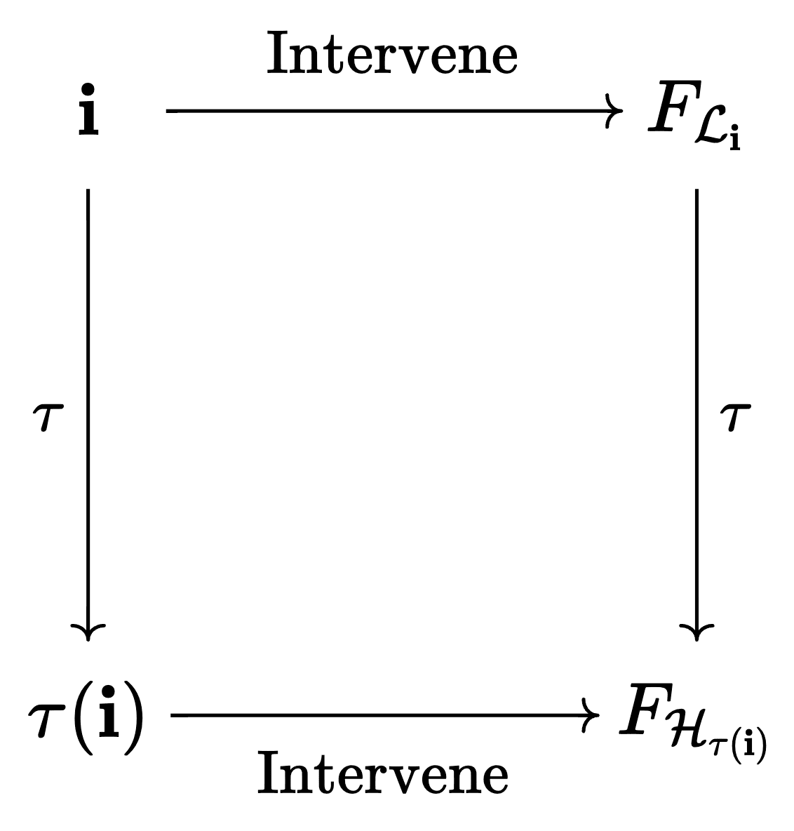
The key idea of causal abstractions is that we can either do an intervention in the low-level model $L$ and then translate the result to the high-level model $H$, or first translate the intervention to $H$ and then perform it there. If $H$ is a good causal abstraction, these two should be equivalent.

There are several somewhat different formalizations of this idea. We follow Geiger et al. (2023) in describing a simplified version of constructive abstraction (Beckers & Halpern, 2019) specifically for deterministic models:

• In addition to $H$ and $\Pi :H\to L$, we also need maps ${\tau }_X:\mathrm{Val}\left({\Pi }_X\right)\to \mathrm{Val}\left(X\right)$ for every high-level node $X\in H$, which map low-level values to high-level values. We write $\tau :\mathrm{Val}\left(L\right)\to \mathrm{Val}\left(H\right)$ for the combination of all these maps. On output nodes, $\tau$ is constrained to be the identity.^[2] 
• The computational graphs $L$ and $H$ induce functions that take their inputs to the joint setting of all their nodes (simply by doing a forward pass). We'll call this function $F_L:\mathrm{Inputs}\left(L\right)\to \mathrm{Val}\left(L\right)$ and $F_H$ analogously.
• For any (hard) intervention $i$ for $L$, i.e. a setting of some of the nodes, we can define the intervened causal graph $L_i$ the usual way. We write $\tau \left(i\right)$ for the corresponding intervention in $H$. If $i$ sets a node $Z\in L$ to value $z$ and $Z$ is in the image of $\Pi$, then $\tau \left(i\right)$ sets  ${\Pi }^{-1}\left(Z\right)$ to $\tau \left(z\right)$. If $Z$ is not in the image of $\Pi$, it is ignored for $\tau \left(i\right)$.
• $(H,\Pi ,\tau )$ is a valid causal abstraction of $L$ if for all interventions $i$, we have

$$F_{H_{\tau \left(i\right)}}=\tau \circ F_{L_i}.$$

We can (somewhat informally) write this as a commutative diagram:

For readers who have seen constructive abstractions described elsewhere, we note that our version might look different because of several simplifying assumptions: we only deal with deterministic acyclic causal graphs, and unlike Geiger et al. (2023) we assume that every node in $H$ corresponds to only one node in $L$. This means that every intervention $i$ in $L$ has some analogous intervention $\tau \left(i\right)$ in $H$ (whereas in the more general version, you need to worry about interventions that do different things to several nodes in $L$ that all correspond to a single node in $H$).

Interchange interventions/Resampling ablations

As we just saw, a causal abstraction consists not only of $H$ and $\Pi$, but also of $\tau$-maps. In the context of neural network interpretability, these would map neural representations to interpretable values in $H$. Specifying these explicitly would be a lot of work—we may instead want to test hypotheses of the form "this neural representation encodes [meaningful feature]" without making claims about how that feature is encoded.

Interchange interventions (Geiger at al., 2021a) let us test hypotheses like that using implicitly defined $\tau$-maps. The idea is that we can generate interventions in $L$ by replacing the activations of some nodes with those on different inputs. Then we get the corresponding intervention in $H$ just by using the same inputs to replace activations in the corresponding nodes.

This is exactly the same idea that's called resampling ablations in the context of causal scrubbing. The full causal scrubbing algorithm has additional components, but it can be understood as using interchange interventions—more on that below.

In the setting for this post, an interchange intervention works as follows:

1. We pick some set of nodes $X_1,\dots ,X_k$ in $L$.
2. We sample a base input $b$ and source inputs $s_1,\dots ,s_k$ from $D$.
3. We fix the values of $X_1,\dots ,X_k$ to the values they would have on $s_1,\dots ,s_k$. For each $X_i$, if $X_i$ is in the image of $\Pi$, then we also fix the corresponding node ${\Pi }^{-1}\left(X_i\right)$ in $H$ to its value on $s_i$.
4. Finally, we compute the values of $L$ and $H$ on the base input $b$, with some values fixed during the forward pass as described in 3.

This procedure lets us generate equivalent interventions on $L$ and $H$ without needing to explicitly compute $\tau$-maps. It's not a complete algorithm though, as we will also need to check whether the effects of these interventions are what the explanation predicts.

The Geiger et al. algorithm

How can we check whether the causal abstraction condition is satisfied using interchange interventions? The answer is that in practice, we don't: we only check a weaker condition. But first, let's understand the key difficulty.

Interchange interventions let us generate matching interventions in both graphs, i.e. pairs $(i,\tau (i\left)\right)$, without explicitly representing or using $\tau$. But if we look at the commutative diagram from above, $\tau$ is also used on the right side to compare the effects of the interventions in the two graphs. It's much less clear how to do that efficiently without representing $\tau$:

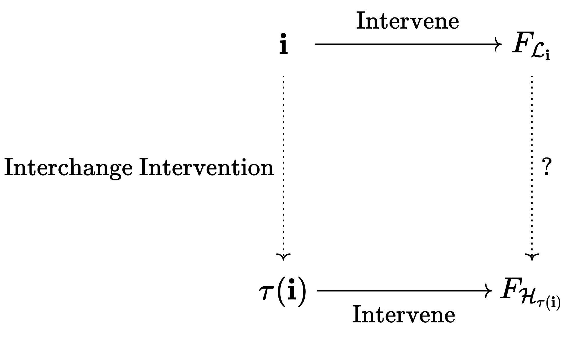
The difference here is that on the left side, we only need to be able to generate lots of matching interventions. But then for each of these interventions, we get some specific values in $L$ and $H$, and we need to decide whether these values match.

So what Geiger et al. do instead is to only compare the outputs of $L$ and $H$ after the interchange intervention. Since we assumed these live in the same space, this is much easier and doesn't require $\tau$-maps.

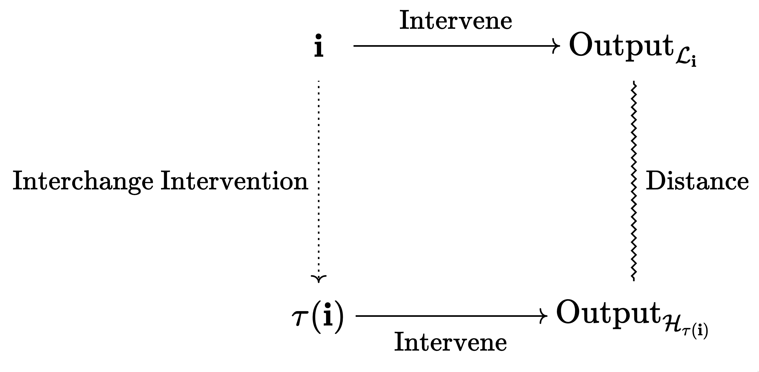
Concretely, Interchange Intervention Accuracy (IIA) (Geiger et al., 2021b) is the probability that the outputs are exactly equal on a random interchange intervention. Of course other metrics are possible, e.g. an expected distance between outputs (as Geiger at al. (2023) point out, IIA is a special case of that with a 0-1-distance).

Because we only compare outputs, an IIA of 100% does not imply that $H$ is a valid causal abstraction.^[3] We will discuss this more and give an example later [LW · GW].

Causal scrubbing

Causal scrubbing also uses interchange interventions (or "resampling ablations"), but the full algorithm differs from the Geiger at al. one in two key ways.

First, causal scrubbing only intervenes in  $L$, not in $H$. So how can we check whether the intervention did what $H$ predicts, without actually intervening on $H$? The answer is simple: we only perform interventions that leave $H$ unchanged. The causal scrubbing algorithm recursively uses rejection sampling to construct interchange interventions that leave all the values in $H$ unchanged. If we perform the corresponding interventions in $L$, that may very well change intermediate activations in $L$. But, if the explanation is correct, it should not change the output of $L$.

So just like the Geiger et al. algorithm, causal scrubbing compares only outputs (as opposed to intermediate values). But because of the restricted space of interventions it performs, it can simply compare the output of $L$ on a base input to the new output after an interchange intervention, instead of comparing to the output of $H$. The only role of $H$ in causal scrubbing is to determine which interventions to perform. Because of that, it's fine for the output type of $H$ to be different than that of $L$ in the case of causal scrubbing. For example, $L$ might output a continuous loss, whereas $H$ only outputs discrete values.

In terms of what we've discussed so far, causal scrubbing would simply perform strictly fewer interventions, and would be a weaker test. However, causal scrubbing has a second key component: treeification of the computational graph.

To understand treeification and why it matters, we'll visualize interchange interventions by mixing colors as in the following figure:

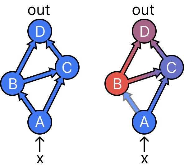
The left figure visualizes a normal forward pass on a single blue input. On the right, we have done an interchange intervention on B that patches in the activation from a red source input. The resulting output D is a mix of both colors, it depends on the blue and the red input.

Now let's look at what happens as we intervene on more nodes simultaneously:

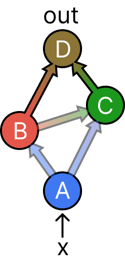
Here, we have performed an interchange intervention on both B and C, using two different source inputs (red and green). The key observation is that the output D now doesn't depend on the blue base input anymore. B and C completely screen off the effects of A on D. In fact, there is no intervention we could perform on this graph where the output would be affected by a mix of three different inputs.

Treeification lets us mix more inputs than a computational graph would ordinarily allow. The idea is that the treeified graph should have the same paths from input to output as the original graph, but separated into a tree:

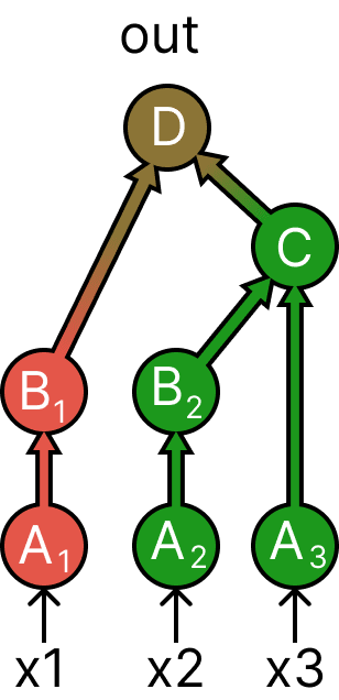
Our graph has three paths from input to output: A-B-D, A-B-C-D, and A-C-D. As you can see, the treeified version has the same paths, but we've made copies of all the nodes as necessary. For example, B occurs in two of the paths, so there are two copies, $B_1$ and $B_2$.

The figure above shows how to do the last interchange intervention we saw on the treeified graph. But because of the treeification we can also do an additional interchange intervention that mixes three different inputs:

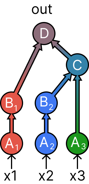
Note that on treeified graphs, we can get any interchange interventions by just computing a forward pass on mixed inputs. We don't actually need to intervene on intermediate nodes: every node has a set of corresponding inputs, and we can just change those inputs without affecting any other downstream nodes. We'll still call this an interchange intervention since it's exactly equivalent in terms of the effects.

Combining what we've discussed so far, causal scrubbing works roughly as follows:

1. Treeify the low-level graph $L$.
2. Sample a base input $b\sim D$ and compute all values in $H$ on input $b$.
3. Perform an interchange intervention on the treeification of $L$ such that the corresponding intervention in the treeification of $H$ would not change any values.
4. Check that the output of $L$ after this interchange intervention (the "scrubbed output") is still the same as before.

There are two subtleties that make this description imprecise:

• The interchange intervention in step 3. is not just any random intervention on the treeified graph. Instead, we intervene as early in the tree as possible, i.e. usually at the inputs. But there's one exception: for nodes that are "unimportant", i.e. not in the image of $\Pi$, we intervene directly on that node. Equivalently, we use the same source input for the entire subtree preceding that node. See here [? · GW] for more discussion on this. The source inputs themselves are just sampled from $D$ as usual.
• Causal scrubbing doesn't actually compare the original and scrubbed output on each base input. Instead, we average both the unchanged and scrubbed outputs over all base inputs and then compare these expectations. In other words, we compute $|E\left[L_{\text{scrubbed}}\right(b,s_i\left)\right]-E\left[L\right(b\left)\right]|$ instead of $E|L_{\text{scrubbed}}(b,s_i)-L\left(b\right)|$. Again see here [? · GW] for a brief discussion on this choice. We will also analyze this more in the next section.

In practice, causal scrubbing can be implemented by a recursive algorithm, as opposed to explicitly constructing the treeification. The resulting recursive call graph corresponds one-to-one to the treeified $L$.

Locally consistent abstractions

Both the Geiger et al. approach and causal scrubbing use interchange interventions to avoid explicitly representing $\tau$-maps. In contrast, locally consistent abstractions (LCAs) do represent $\tau$-maps explicitly. In practice, $\tau$-maps will likely not be specified as part of an interpretability hypothesis. Instead, they can be learned: if there is any $\tau$-map for which an explanation $H$ would be valid, then we accept $H$. The only constraint is that, as for causal abstractions, the $\tau$-map on output nodes must be the identity.

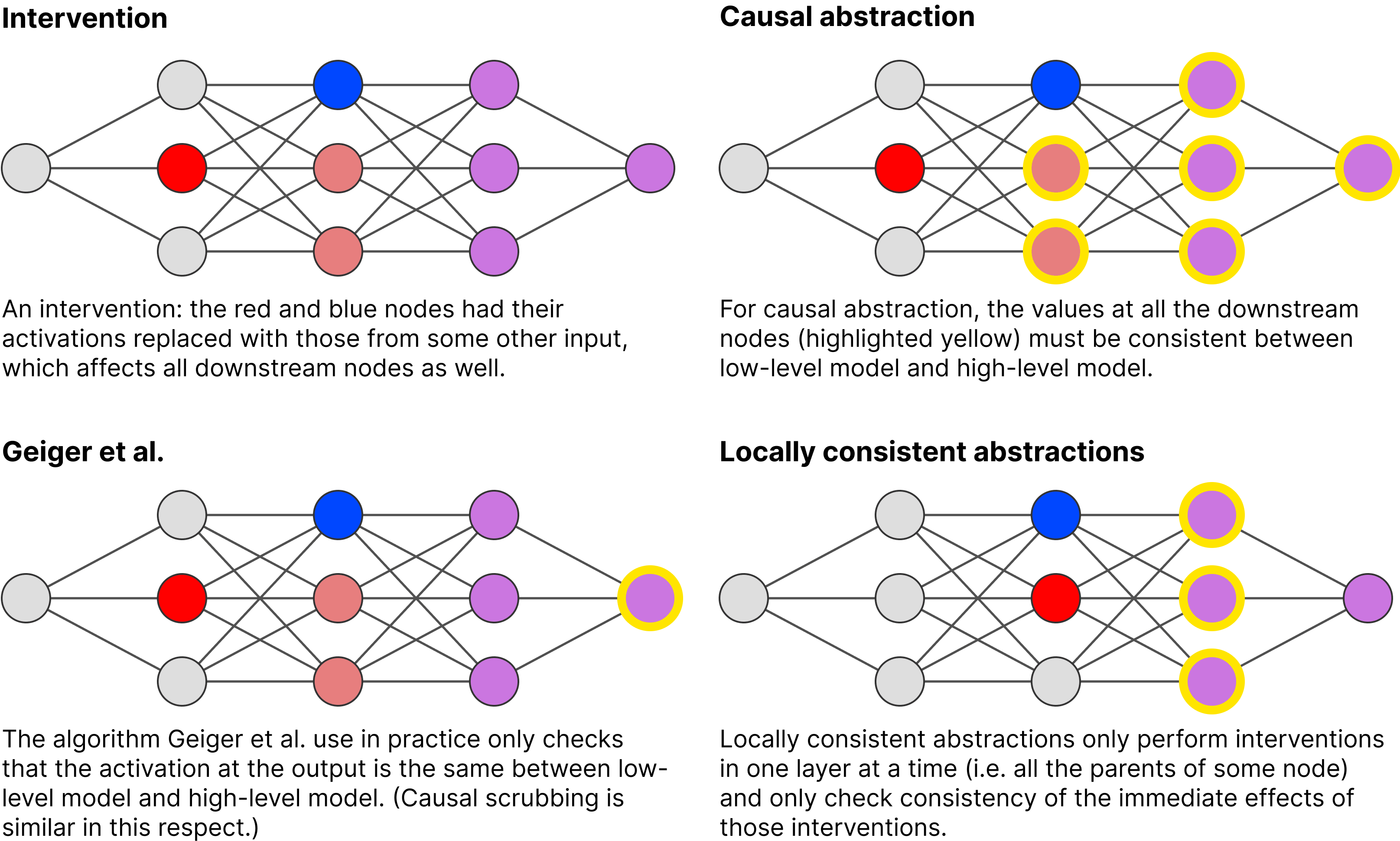
The other key difference is that LCAs only check whether the immediate effects of an intervention are the same between low-level model and high-level model. In this sense, they can be seen as simplifying causal abstraction in another direction than Geiger et al. or causal scrubbing do:

• Full-blown causal abstractions check consistency of interventions on all variables.
• Geiger et al. and causal scrubbing only check the consistency of the output.
• LCAs only check the consistency of the immediate children of the node we intervened on.

The following figure contrasts those approaches, the nodes for which consistency is checked are circled in yellow:

Let's describe LCAs more formally in their own right. For any node $X$, we'll write $f_X$ for the function that computes the value of $X$ from its parents. Then $(H,c,\tau )$ is a locally consistent abstraction if for every node $X$ in $H$, we have

$$f_X\circ \tau =\tau \circ f_{{\Pi }_X}.$$

We are abusing notation slightly here, see footnote.^[4] We can write this as a commutative diagram again:

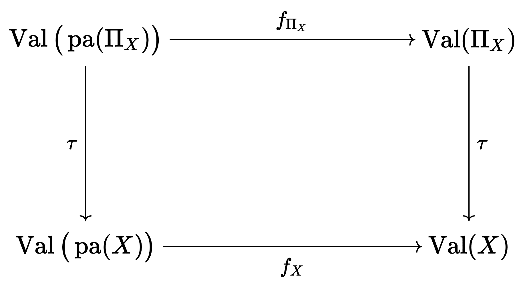
$\mathrm{pa}\left(X\right)$ are the parents of node $X$ and $\mathrm{Val}\left(X\right)$ the set of possible values $X$ can take, analogously for the other cases.

Intuitively, this is saying we can either perform a computational step in the low-level model ($f_{{\Pi }_X}$) and then abstract with $\tau$, or we can first abstract and then perform a computational step in the high-level model ($f_X$). For good abstractions, these should be equivalent.

We haven't explicitly mentioned interventions here. Simply computing $f_X$ is of course equivalent to intervening on $\mathrm{pa}\left(X\right)$ and then evaluating $X$, but the language of causality and interventions isn't really necessary if we only want to describe local consistency.

So far, we've simply stated the consistency condition as equality of two functions. But realistically, we often can't check exact equality, we can only test the consistency condition on samples (like in the earlier methods). There are two options for how to get activations for $\mathrm{pa}\left({\Pi }_X\right)$:

1. Sample a single input to $L$ and compute all activations from that one input.
2. Sample a separate input for each parent.

(Of course, yet other options exist, e.g. computing all "unimportant" parents from a single input but all important parents from different ones, similar to causal scrubbing.)

Finally, note that if the consistency condition was satisfied exactly and on all possible inputs, then this would also imply global consistency in the causal abstraction sense. But with restricted activation distributions, and with approximate consistency, local and global methods differ in several aspects. We'll discuss this more in the next section. 

Axes of differences between methods

Hopefully, you now have a sense of the differences between causal abstraction, the specific implementation by Geiger et al., causal scrubbing, and LCAs. In this section, we'll identify several "themes" in how these methods differ, and discuss the consequences of those differences.

Set of accepted explanations

Throughout this discussion, we'll be asking: "How strict is this notion of correctness, i.e. which explanations does it accept?" Here are the results upfront:

• If an explanation is a causal abstraction, then it is also an LCA and accepted by the Geiger et al. algorithm.
• There are probably no other implications, i.e. for any other pair of methods, there are some explanations that method A accepts but method B rejects, and some explanations where it's the other way around. ("Probably" because we haven't formally written down counterexamples for all the pairs yet, but it seems fairly clear.)

It's not obvious that we always want the strictest possible definition—we'll briefly discuss this question later.

Checking consistency for intermediate nodes vs output only

Causal abstraction and LCA check consistency conditions for intermediate nodes of the computational graphs, whereas the concrete Geiger et al. algorithm and causal scrubbing only look at the output.

Looking only at the output means accepting some weird explanations that causal abstractions and LCA would reject. For example, say that the output node of both $L$ and $H$ is simply constant. In that case, $H$ can have arbitrary circuits before the output and will be accepted as a correct explanation. A constant output is an extreme case, but similar things can happen much more generally: $H$ can have "hallucinated circuits" as long as they don't actually impact the final output.

Having mechanisms in $H$ that don't affect the output is a strange property, and perhaps we could rule out such explanations a priori (e.g. by favoring simpler explanations). We don't know whether such an approach could fully bridge the gap between output-based methods and causal abstraction.

Explicit vs implicit $\tau$-maps

Whether to represent $\tau$-maps explicitly is mostly a choice of implementation that affects what you can efficiently do. The explicit $\tau$-maps are what allow LCAs to compare intermediate nodes, as we just discussed. On the other hand, there is of course some overhead from learning these maps, and the practical difficulty of optimizing them may reject extra hypotheses.

Global vs local consistency and activation distributions

All methods except LCA check the effects of interventions on nodes that are arbitrarily far downstream, i.e. they check global consistency. One of the effects of that is that they check consistency on activations that are "off-distribution", i.e. not induced by forward passes on the input distribution $D$.

Off-distribution activations arise in a two-step process:

1. We compute activations for two nodes $n_1$ and $n_2$ on different inputs $x_1$ and $x_2$ (because of an interchange intervention). At this point, the overall state of the computation might already be off-distribution: normally, $n_1$ and $n_2$ would both be computed from the same input, and computing them from different inputs might have destroyed some mutual information between them. But the activation of individual nodes is still on-distribution.
2. Now assume $n_1$ and $n_2$ share a common child (or later descendant). The activations of $n_1$ and $n_2$ may be a combination that could never occur on normal forward passes. In that case, the activation of the common child could also be one that is not induced by any single input. So now even individual activations are off-distribution.

We can get the step 1. off-distribution activations quite easily for LCA by sampling activations for parents in $L$ using separate inputs. Step 2. off-distribution activations might then occur in the node $X$ for which we're checking consistency, but crucially, these activations won't be fed into any other mechanisms $f_Y$, only into $\tau$. So we're only testing the causal mechanisms $f_X$ on-distribution (at least in terms of the marginal distribution for each input to $f_X$).

This leads to LCA accepting some explanations that all the other methods reject. A typical example is a node $X$ in $L$ that has the same value $v_1$ on all inputs from $D$, but a different value $v_2$ on other inputs. LCA will accept certain explanations that claim $X$ is mechanistically constant (as opposed to being computed by some complicated mechanism that happens to always give the same result). The other methods will sometimes reject such an explanation, depending on the actual implementation of $X$. 

A related example are duplicate mechanisms in $L$: if $L$ has two copies of the same circuit and then just takes the average at the end, LCA will often accept an explanation that only points out one of the circuits, while the other methods will reject that explanation.

Only allowing interventions that leave $H$ unchanged

Recall that causal scrubbing only allows interventions that don't change any of the values in the explanation $H$. This leads to examples where causal scrubbing accepts an explanation that all the other methods reject. Consider the following type of explanation $H$:

• There is a node in $H$ for every node in $L$.
• All nodes in $H$ are simply the identity—they just store the values of all their parents.

Effectively, $H$ doesn’t do anything, it just keeps the input around indefinitely. But causal scrubbing always accepts this “explanation”: since $H$ claims that all the nodes matter, and that all the information in every node matters, it doesn’t allow any ablations at all.

Expectations vs sample-wise errors

Causal scrubbing compares the expectations of the scrubbed output and the original one, whereas all the other methods compute errors for each base input and then take the expectation over these errors. The second approach is stricter in terms of which explanations are accepted. With the causal scrubbing metric, errors can "cancel", see here [LW · GW] for an example.

Treeification

Treeification is the one way in which causal scrubbing is stricter than all the other methods. Recall the figure above where we showed how treeification allows "mixing" more different inputs than is possible using only interventions on the original graph. In some cases, this should mean causal scrubbing will test on activations that causal abstractions doesn't generate, so it may reject explanations that fail on these activations.

Computational complexity

Because of the (implicit) treeification, computing a single scrubbed output for causal scrubbing can take time exponential in the size of the explanation $H$. In contrast, LCA and interchange interventions on non-treeified graphs take linear time.

One subtlety is that there are exponentially many different interventions one could sample in the Geiger et al. approach. In practice, sampling only a reasonably small number of interventions plausibly seems good enough, but we're not entirely sure to what extent that retains benefits of doing global interventions.

One could also use approximations of causal scrubbing that only trace out a small random part of the treeification of $L$, to avoid exponential time complexity. Again, we don't know whether this would preserve the higher strictness that treeification usually gives.

While LCAs are linear time in the size of $L$ and $H$, there are two caveats:

• In the worst case, computing the $\tau$-maps can be cryptographically hard: assume that the activation of some node in $L$ is a one-way permutation of the input, and the activation of the corresponding node in $H$ is just the input (i.e. that nodes implements the identity). Forward passes of $H$ and $L$ are cheap, but computing the $\tau$-map for this node pair corresponds to inverting the one-way permutation.
• In practice, learning the $\tau$-maps will add some overhead. This overhead might be reasonably small if e.g. linear $\tau$-maps suffice and the explanation is significantly smaller than the full network.

Compounding errors and chaotic computations

The examples so far showed discrepancies between methods in terms of when they judge an explanation as perfectly correct. There is one additional qualitative difference once we consider graded judgments of how incorrect an explanation is. Namely, LCAs compute local errors, which don’t compound throughout the computation. To get a single metric, we just add up all the local errors. For all the other methods, if an intervention early on in the computation has slightly different effects than predicted by $H$, these effects can compound to get a very large error.

This difference becomes very pronounced if $L$ implements a chaotic computation. For example, say that $L$ simulates a double pendulum using 64-bit floating point numbers, and $H$ implements the exact same computation using 32-bit floating point numbers. Under LCAs, this explanation has only a rather small error. In contrast, the explanation is completely wrong according to causal scrubbing or interchange intervention accuracy, assuming the simulation runs for long enough that 32-bit errors compound a lot.

Multiple simultaneous interventions

Earlier versions of interchange interventions allowed interventions encompassing only a single abstract node at a time. This leads to accepting some incorrect hypotheses that are rejected by causal scrubbing and by later versions of interchange interventions, see the  appendix for an example. The problems don’t seem specific to interchange interventions, and multiple simultaneous interventions seem desirable for any similar method. In their latest versions, all methods reject these types of examples.

Discussion

"I" in this section refers to Erik and these are specifically my personal takes.

A common framework

Causal abstractions seem like a promising way of unifying all these approaches. LCAs and the Geiger et al. approach can both be seen as weakening the causal abstraction condition in different ways. And causal scrubbing is still very similar except for working on the treeified graphs.

On the other hand, I do think there's room for several different frameworks or perspectives here. For example, LCAs don't actually have a very causal feel, but seem very natural to me from other perspectives.

Combining components in different ways

My sense is that the specific algorithms people have come up with are largely historical accidents, and you could just as well combine some of the components in different ways. For example, the choice of comparing expectation or sample-wise errors has nothing to do with whether you want to do treeification.

It's not entirely arbitrary that the purely local method (LCA) uses explicit $\tau$-maps and the others don't (since local consistency checks require $\tau$-maps, whereas if you check global effects of interventions, you can just look at the output). But I think you could totally have both explicit $\tau$-maps and global consistency checks, if that's the level of strictness you want (and you're willing to pay a bit of computational overhead). That would exactly correspond to causal abstraction.

How strict do we want our criterion to be?

Given that the different methods all seem incomparable, we could get a particularly strict criterion by only accepting if all of them accept (or by directly doing full-blown causal abstraction on treeified graphs).

It's not clear to me that we should though:

• For interpretability, being stricter also means it's harder to find an acceptable explanation (or your explanation might have to be bigger because it has to include more parts of the network).
• I think the benefits of the specific ways in which some of these methods are stricter than others are very poorly understood. Hopefully, strictness helps accepted explanations generalize to out-of-distribution inputs, but we don't really know to what extent that's true.
  • If your goal with interpretability is literally to edit activations during forward passes (i.e. do interventions), then that's a strong argument for testing global effects of interventions. But if you just want to use your explanation to figure out OOD behavior of your network, then it's far from obvious to me why one of these methods in particular is the right one.
• For mechanistic anomaly detection, you want your explanation to fail on some out-of-distribution inputs. Being too strict could mean you force the explanation to contain the anomalous mechanism you want to detect (in which case detection won't work).

Different conceptual goals

I think of the global approaches (causal scrubbing/interchange interventions) as trying to only accept explanations that contain all the mechanisms relevant for the input-output behavior. So for example, if there are two copies of a mechanism, both need to be included in the explanation. On the flip side, causal scrubbing and the Geiger et al. approach, because they only look at the output, will accept some explanations that "hallucinate" additional mechanisms.

LCAs accept an explanation as long as it is sufficient to explain the output and contains at most the mechanisms that are actually present. So if there are two exact copies of a mechanism (that e.g. get averaged at the end), it will accept an explanation that only contains one of them. But if the explanation contains hallucinated mechanisms, it will be rejected.

Full causal abstraction combines both of these, accepting an explanation only if it contains exactly the mechanisms that are important for the output (and potentially irrelevant ones, but not hallucinated ones). A big caveat though is that I'm pretty confused about how "important for the output" should be interpreted if we only want to explain behavior on some distribution $D$. As long as we aren't literally interested in interventions (i.e. only care about behavior on actual inputs), it's not obvious that e.g. a second copy of a mechanism is "important for the output".

Conclusion

On the one hand, we have seen that causal scrubbing, causal abstractions, and locally consistent abstractions are more similar than they may appear based on their original expositions. In practice, it seems likely they will often give similar results.

On the other hand, there are differences between all of these methods, and each one of them accepts some hypotheses that are rejected by one of the other methods. We could combine all of them to get one stricter definition of "correct explanations". However, the differences between the approaches highlight conceptual questions about what it means to explain a behavior "on a distribution", so it's not obvious that getting the strictest definition we can is desirable.

Appendix

Early papers in the Geiger et al. line of work only allowed for one abstract node to be intervened on at a time, which makes the method less strict.

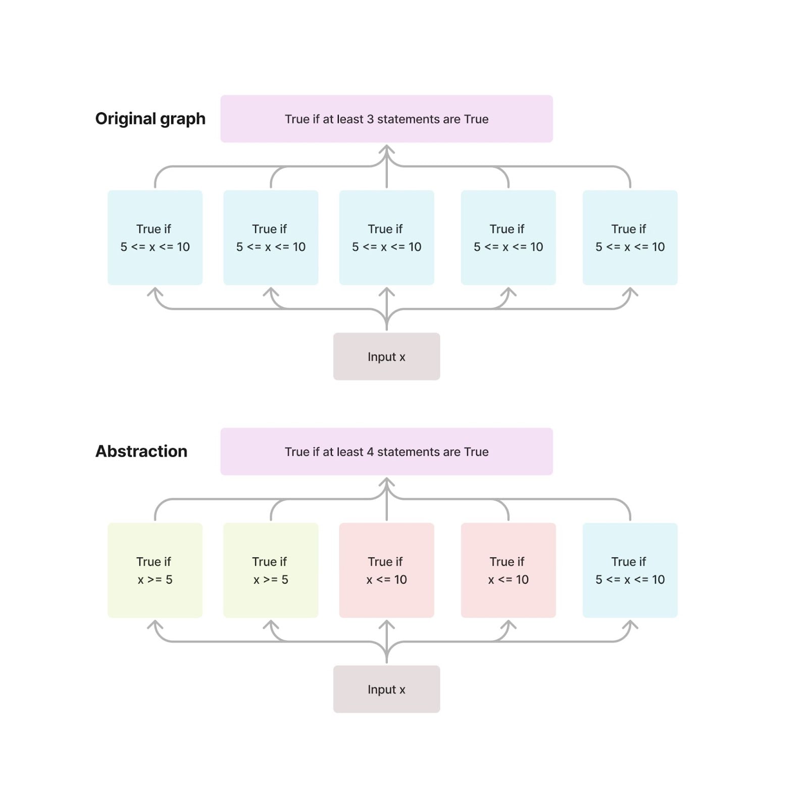
For instance, consider an example where we have numerous copies of the same computation stacked together in a graph $L$, while the output of $L$ is a value produced by the majority of copies (which will always be the same without interventions). We can come up with abstractions for each of these duplicates that are individually performing distinct tasks, but together perform a computation that is a seemingly perfect causal abstraction of $L$, if we’re only allowed to perform one intervention at a time.

For a concrete example, consider the following figure:

Here for any base input $b$ and source input $s$ and any node $X\in L$ to be intervened on, the output of $L$ after the intervention is $I[5\le b\le 10]$. We'll show this is also true for $H$. 

If the intervention is on a yellow node, $H$ outputs

$$\{\begin{array}{cc}\text{True},& I[s\ge 5]+I[b\ge 5]+I[b\le 10]+I[b\le 10]+I[5\le b\le 10]\ge 4\\ \text{False},& \text{otherwise}\end{array}$$

If $5\le b\le 10$, then this expression is true. If $b<5$, then the 2nd and the 5th indicators are false and the whole expression is false. If $b>10$, then the 3rd and 4th indicators are false. So the output of $H$ matches $L$ for interventions on one of the yellow nodes, and analogously for the red nodes.

It's also obvious that the output of $H$ on a blue intervention is $I[5\le b\le 10]$ since if $5\le b\le 10$, then the first four indicators are true, otherwise at least 2 of them are false.

Therefore, this abstraction would be accepted by doing interchange interventions that intervene on only one node at a time. On the other hand, causal scrubbing or causal abstractions with multiple interventions don’t accept this abstraction (as long as the input distribution isn't too impoverished).^[5]

We came up with this example while figuring out to what extent multiple interventions are necessary. Turns out even in a very simple setting with 5 nodes, methods that allow only one intervention might fail. We therefore think it is necessary for all further intervention methods to permit multiple simultaneous interventions. 

1. ^{^}

   Some versions of causal scrubbing allow the correspondence $\Pi$ to map vertices $u,v\in H$ with an edge $u\to v$ to non-adjacent ${\Pi }_u,{\Pi }_v$, so long as a path from ${\Pi }_u$ to ${\Pi }_v$ exists; which is technically not a graph homomorphism. This post follows the published setup for causal scrubbing, and restricts $\Pi$ to be a graph homomorphism.

2. ^{^}

   Recall that we assume $H$ and $L$ have the same output type, so the identity function makes sense. If we didn't constrain the $\tau$-maps on outputs, an explanation could choose a constant $\tau$-map for the output, and thus wouldn't actually need to explain anything. As mentioned in the Setup section, if we only want $H$ to explain some aspect of the output, we make that choice a part of $L$.

3. ^{^}

   Note that Geiger et al., (2021b) have a result showing that 100% IIA does imply a valid causal abstraction. However, this is for a high-level model where all but one intermediate node have been marginalized. We are saying that the full high-level model $H$ with multiple intermediate nodes need not be a causal abstraction.

4. ^{^}

   The two copies of $\tau$ are really defined over different domains, and there should technically be a projection map that discards the values of any "unimportant" parents, i.e. those that don't have corresponding nodes in $H$. So the more pedantic version would be

   $$f_X\circ {\tau }_{\mathrm{pa}\left(X\right)}\circ {\pi }_{\Pi \left(\mathrm{pa}\right(X\left)\right)}={\tau }_X\circ f_{{\Pi }_X},$$

   where $\mathrm{pa}\left(X\right)$ is the set of parents of $X$.

5. ^{^}

   Consider, for instance, causal scrubbing with a uniform distribution $D$ over $\{1,7,18\}$. Note this example would work with other input spaces that have at least one value below 5, above 10 and in the interval [5, 10] each, but for simplicity we consider the minimal possible input space.

   It is clear that $E_{x\sim D}\left[L\right(x\left)\right]=\frac{1}{3}$. At the same time, the scrubbed expectation would equal $E\left[L_{\text{scrubbed}}\right]=\frac{11}{48}\ne \frac{1}{3}$: if $b=1$, then the value of the yellow nodes is False. There is only one value in $D$ that agrees with $b$ on yellow nodes, which is 1. Thus, the value of the first two nodes in G shall be false. Similarly, the value of the 5th node is also False and $L_{\text{scrubbed}}(b,s)=0$. The same argument works if $b=18$. If $b=7$, then both 7 and 18 agree on yellow nodes, so the value of the first two nodes in G is equally probably either True or False. Same for the 3rd and 4th nodes. The 5th node is always True. Since the output of G is the majority of nodes, it will output True in $(\frac{4}{2})+(\frac{4}{3})+(\frac{4}{4})$ = 11 cases. Thus, the scrubbed expectation equals $E_{\text{scrubbed}}=\frac{1}{3}\cdot 0+\frac{1}{3}\cdot 0+\frac{1}{3}\cdot \frac{11}{16}=\frac{11}{48}$.

3 comments

Comments sorted by top scores.