Exploring SAE features in LLMs with definition trees and token lists

post by mwatkins · 2024-10-04T22:15:28.108Z · LW · GW · 5 comments

Contents

  Introduction
    Objective
    Tool overview
  Functionality 1: Generating definition trees
    How it works
    Examples 
      Striking success: Layer 12 SAE feature 121 
      Less successful: Layer 6 SAE feature 17
  Functionality 2: Closest token lists
    How it works
    Examples 
      Striking success: Layer 0 SAE feature 0
      Another success: Layer 0 SAE feature 7
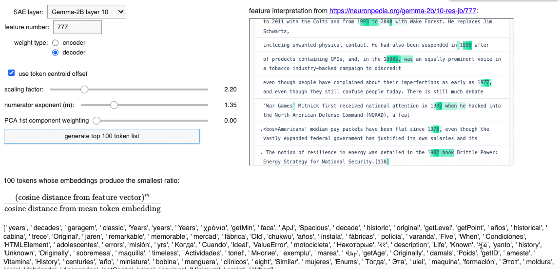
      A partial success: Layer 10 SAE feature 777
      Observations
  Discussion and limitations
  Future directions
  Appendix: Further successful examples
None
5 comments

TL;DR A software tool is presented which includes two separate methods to assist in the interpretation of SAE features. Both use a "feature vector" built from the relevant weights. One method builds "definition trees" for "ghost tokens" constructed from the feature vector, the other produces lists of tokens based on a cosine-similarity-based metric.  

Links: Github repository, Colab notebook

Thanks to Egg Syntax [LW · GW] and Joseph Bloom [LW · GW] for motivating discussions.

Introduction

Objective

The motivation was to adapt techniques I developed for studying LLM embedding spaces (in my series of "Mapping the Semantic Void" posts [1 [LW · GW]] [2 [LW · GW]] [3 [LW · GW]]) to the study of features learned by sparse autoencoders (SAEs) trained on large language models (LLMs). Any feature learned by an autoencoder corresponds to a neuron in its single hidden layer, and to this can be associated a pair of vectors in the LLM's representation space: one built from its encoder layer weights and one from its decoder layer weights.

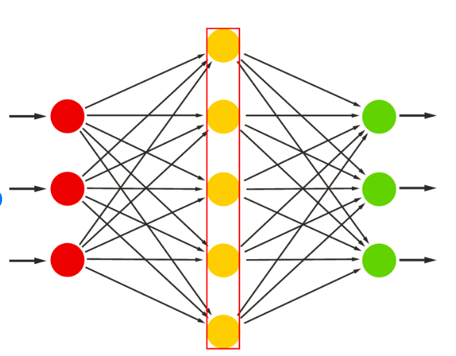
In my earlier work I used custom embeddings in order to "trick" LLMs into "believing" that there was a token in a tokenless location so I could then prompt the model to define this "ghost token". As this can be done for any point in the model's representation/embedding space, it seemed worth exploring what would happen if SAE feature vectors were used to construct "ghost tokens" and the model were prompted to define these. Would the definitions tell us anything about the learned features?

I focussed my attention on the four residual stream SAEs trained by Joseph Bloom on the Gemma-2B model, since data was available on all of their features via his Neuronpedia web-interface.

Tool overview

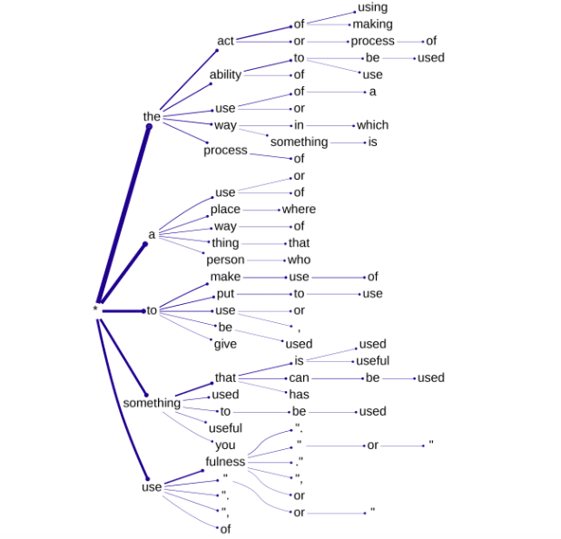
The first method I explored involved building "definition trees" by iteratively prompting Gemma-2B with the following and collecting the top 5 most probable tokens at each step.

A typical definition of "<ghost token>" would be "

The data is stored as a nested dictionary structure and can be displayed visually as a tree diagram which, with its branching/"multiversal" structure provides an interestingly nonlinear sense of meaning for the feature (as opposed to an interpretation given via a linear string of text).

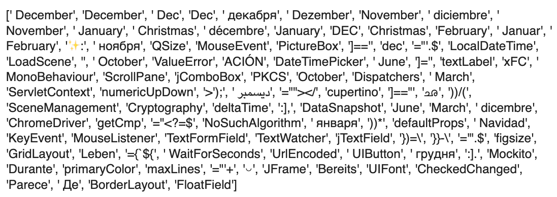
In the second method, the model itself is not even used. No forward passes are necessary, all that's needed are the token embeddings. The initial idea is to look at which tokens' embeddings are at the smallest cosine distance from the feature vector in the model's embedding/representation space (those which are "cosine-closest"). The problem with this, as I discovered when exploring token embedding clusters in GPT-3 (the work which surfaced the so-called glitch tokens) [LW · GW], is that by some quirk of high-dimensional geometry, the token embeddings which are cosine-closest to the mean token embedding (or centroid) are cosine-closest to everything. As counterintuitive as this seems, if you make a "top 100 cosine-closest tokens" list for any token in the vocabulary (or any other vector in embedding/representation space), you will keep seeing the same basic list of 100-or-so tokens in pretty much the same order. 

In order to filter out these ubiquitously proximate tokens from the lists, it occurred to me to divide the cosine-distance-to-the-vector-in-question by the cosine-distance-to-the-centroid and look for the smallest values. This incentivises a small numerator and a large denominator, thereby tending to exclude the problem tokens which cluster closest to the centroid. And it works quite well. In fact, it's possible to refine this by raising the numerator to a power > 1 (different powers produce different "closest" lists, many topped by a handful of tokens clearly relevant to the feature in question).

Functionality 1: Generating definition trees

How it works

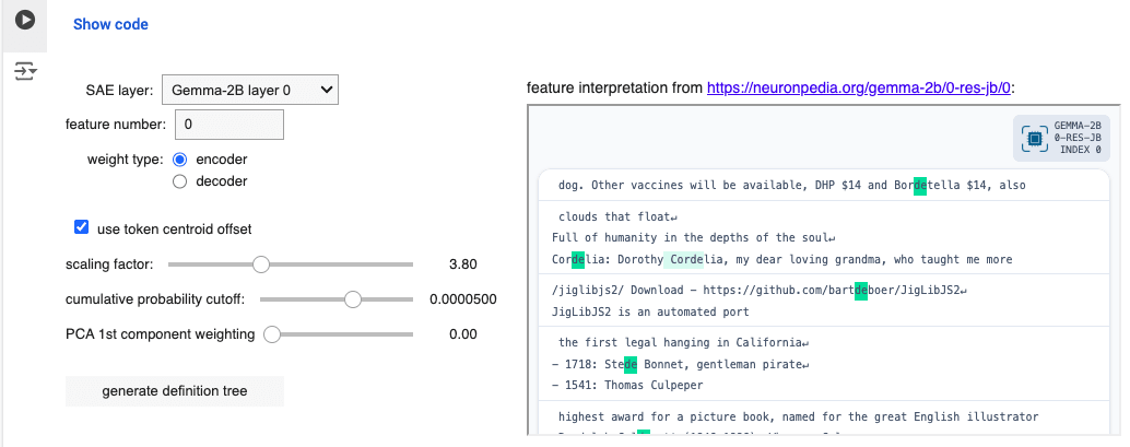
The user selects from a dropdown one of the four Gemma-2B SAEs available (trained on the residual stream at layers 0, 6, 10 and 12), enters a feature number between 0 and 16383 and chooses between encoder and decoder weights. This immediately produces a feature vector in the model's representation space. We're only interested in this as a direction in representation space at this stage, so we normalise it to unit length.

The PCA weighting option can be used to modify the direction in question using the first component in the principal component analysis of the set of all token embeddings. We replace our normalised feature vector with

$(1-w)\ast \text{normalised feature vector}+w\ast {\text{PCA}}_1$

so that if $w=0$ the feature vector is unaffected. The resulting vector is then normalised and scaled by the chosen scaling factor. 

If the "use token centroid offset" checkbox is left in its default (True) setting, the rescaled feature vector is added to the mean token embedding. No useful results have yet been seen without this offset.

The default value of 3.8 for the scaling factor is the approximated distance of Gemma-2B token embeddings from the mean token embedding (centroid), so by using the centroid offset and a value close to 3.8, we end up with something inhabiting a typical location for a Gemma-2B token embedding, and pointing in a direction that's directly tied to the encoder or decoder weights of the SAE feature that was selected.

The embedding of an arbitrary, little-used token is then overwritten with this 2048-d vector (actually a shape-[2048] tensor), and this customisation allows the forward passing through the model of prompts including this "ghost token". Prompting for a typical definition of "<ghost token>" and taking the top 5 logits at each iteration allows for the construction of a tree of definitions, encoded as a nested dictionary where each node records a token and a cumulative probability (product of probabilities of all output tokens thus far along that branch). 

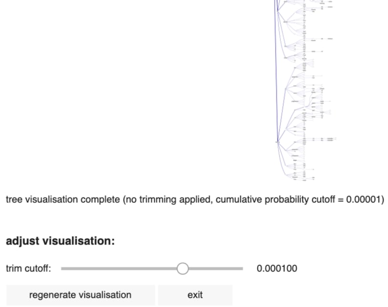
The "cumulative probability cutoff" parameter determines below which threshold a branch on the definition tree gets terminated. Larger values therefore result in small trees. There is a point below which the tree visualisation output becomes too dense to be visually useful, but the interface allows "trimming" of trees to larger cutoff values:

 

Examples 

Striking success: Layer 12 SAE feature 121 

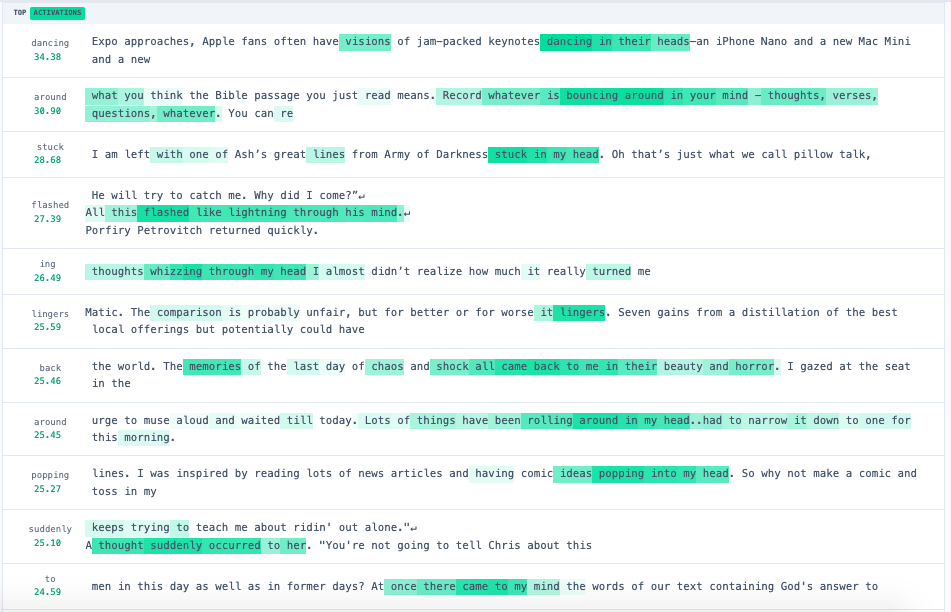
This feature is activated not so much by specific words, usages or syntax as the general notion of mental images and insights, as seen in the following top activating text samples found for this feature (from Neuronpedia):

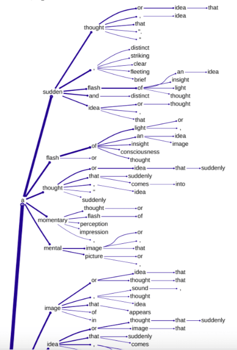
Here's the uppermost part of the definition tree (using cumulative probability cutoff 0.00063, encoder weights, scaling factor 3.8, centroid offset, no PCA)

 

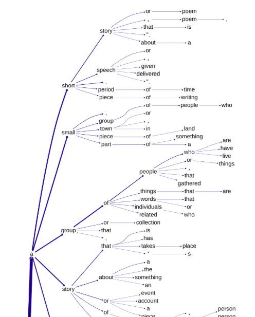
Less successful: Layer 6 SAE feature 17

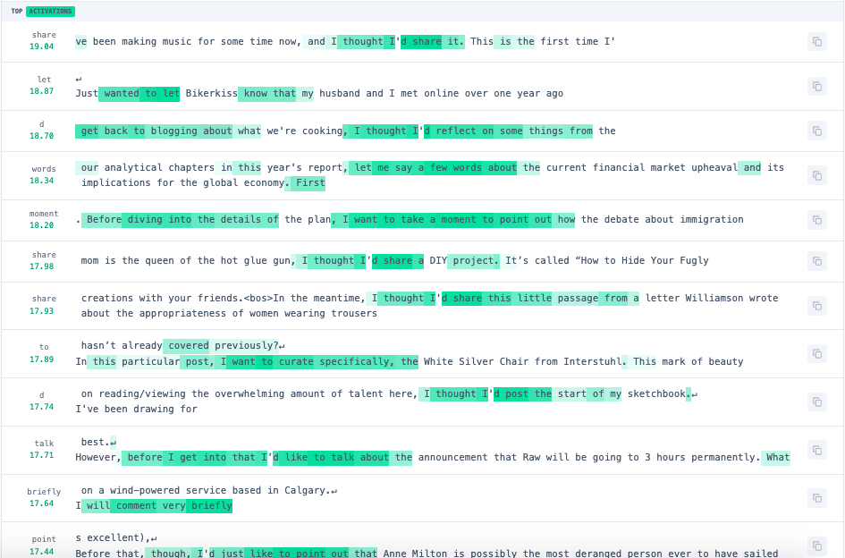
This feature is activated by references to making short statements or brief remarks, as seen in the following top activating text samples found for this feature (from Neuronpedia):

Here's the uppermost part of the definition tree (using cumulative probability cutoff 0.00063, encoder weights, scaling factor 3.8, centroid offset, no PCA). There's clearly some limited relevance here, but adjusting the parameters, using decoder weights, etc. didn't seem to be able to improve on this:

 

Functionality 2: Closest token lists

How it works

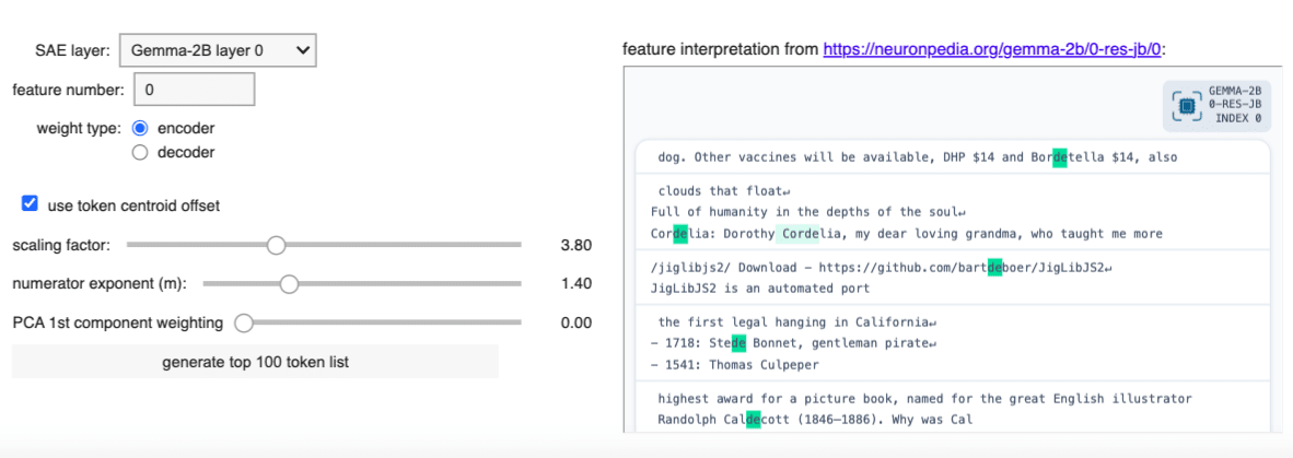
As with functionality 1, the user chooses an SAE, a feature number and whether to use encoder or decoder weights. From these, a feature vector is immediately constructed. It will then be modified by the scaling factor and/or choices to use (or not use) token offset or first PCA direction. The resulting vector in representation space is then used to assemble a ranked list of 100 tokens which produce the smallest value of 

$\left(\text{cosine distance from feature vector}{)}^m/\right(\text{cosine distance from token centroid})$

where the exponent $m$ is chosen by the user. This trades off the desired "cosine closeness" with the need to filter out those tokens which are cosine-closest to the centroid (and which would otherwise dominate all such lists as mentioned above).

Examples 

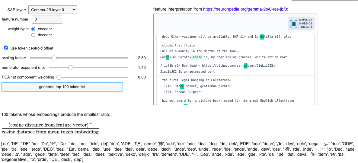
Striking success: Layer 0 SAE feature 0

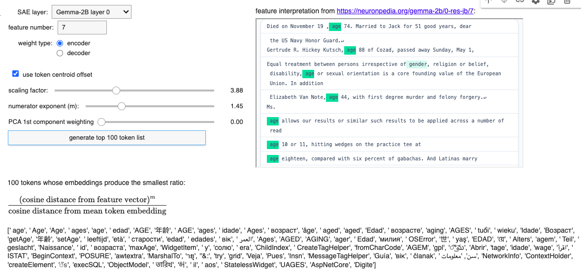
Another success: Layer 0 SAE feature 7

A partial success: Layer 10 SAE feature 777

Observations

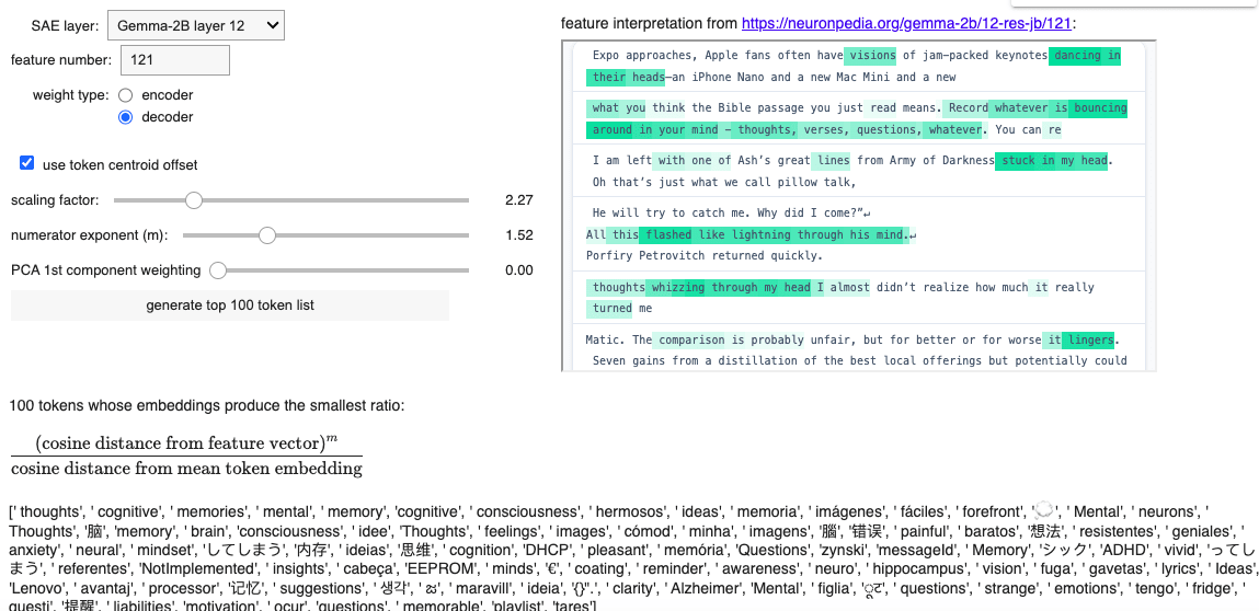
When a learned SAE feature is one which seems to activate on the occurrence of a particular word or sequence of letters, the token list method is particularly effective, producing the tokens you would expect. But more nuanced features can also produce relevant lists with some parameter experimentation, as with layer 12 SAE feature 121 seen earlier (concerned with mental states):

Discussion and limitations

One obvious issue here is that producing relevant trees or lists often involves some experimentation with parameters. This makes their use in automated feature interpretation far from straightforward. Possibly generating trees and lists for a range of parameter values and passing the aggregated results to an LLM via API could produce useful results, but tree generation at scale could be quite time-consuming and compute-intensive.

It's not clear why (for example) some features require larger scaling factors to produce relevant trees and/or lists, or why some are more tractable with decoder-based feature vectors than encoder-based feature vectors. This may seem a weakness of the approach, but it may also point to some interesting new questions concerning feature taxonomy.

Future directions

There is significant scope for enhancing and extending this project. Some possibilities include:

Adaptation to other models: The code could be easily generalised to work with SAEs trained on other LLMs.
Improved control integration: Merging common controls between the two functionalities for streamlined interaction.
Enhanced base prompt customisation: Allowing customisation of the base prompt for the "ghost token" definitions (currently '''A typical definition of "<ghost token>" would be''').
Expanded PCA and linear combination capabilities: Exploring the impacts of multiple PCA components and linear combinations of encoder- and decoder-based feature vectors.
API integration for feature interpretation: Exporting outputs for further interpretation to LLMs via API, enabling automated analysis.
Feature taxonomy and parameter analysis: Classifying features according to the efficacy of these two tools in capturing the types of text samples they activate on, as well as the typical parameter settings needed to produce relevant effective outputs.

I'm most excited about the following, probably the next direction to be explored:

Steering vector and clamping applications: Leveraging feature vectors as "steering vectors" and/or clamping the relevant feature at a high activation in the tree generation functionality to direct the interpretive process, almost certainly enhancing the relevance of the generated trees.

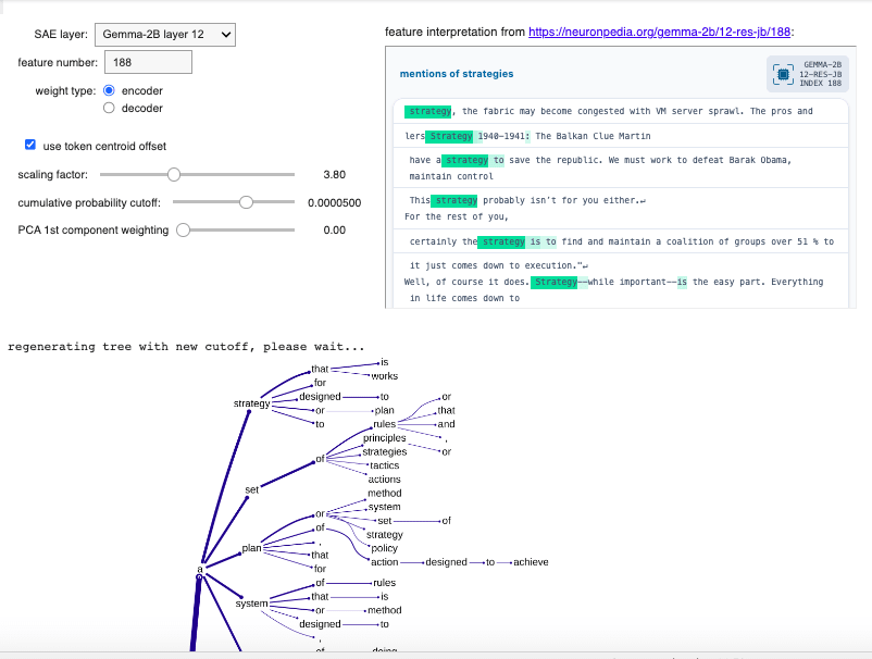
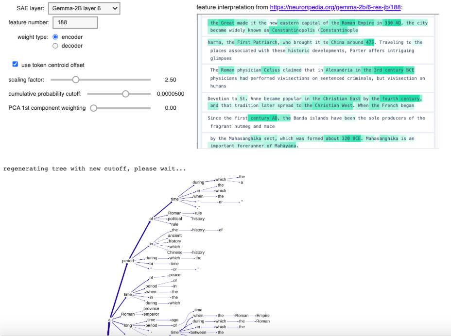
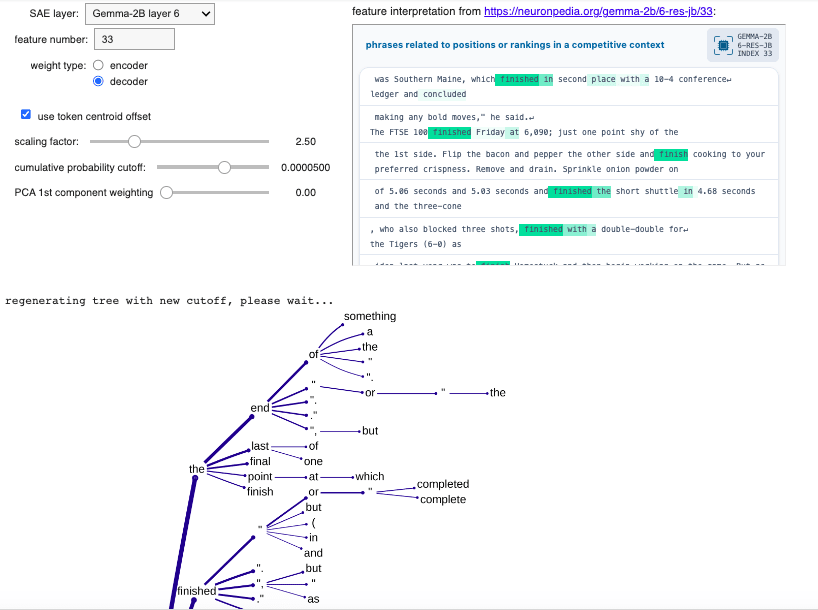
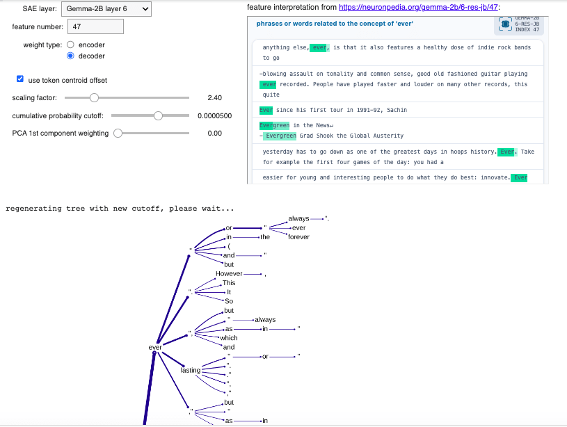
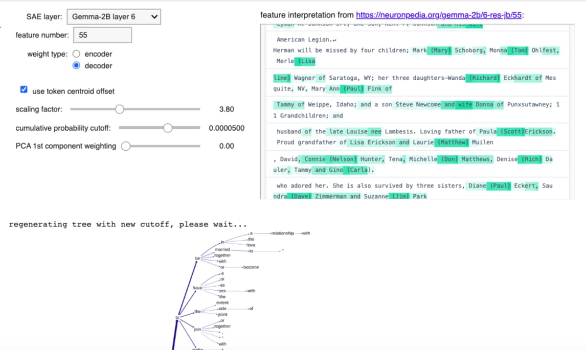
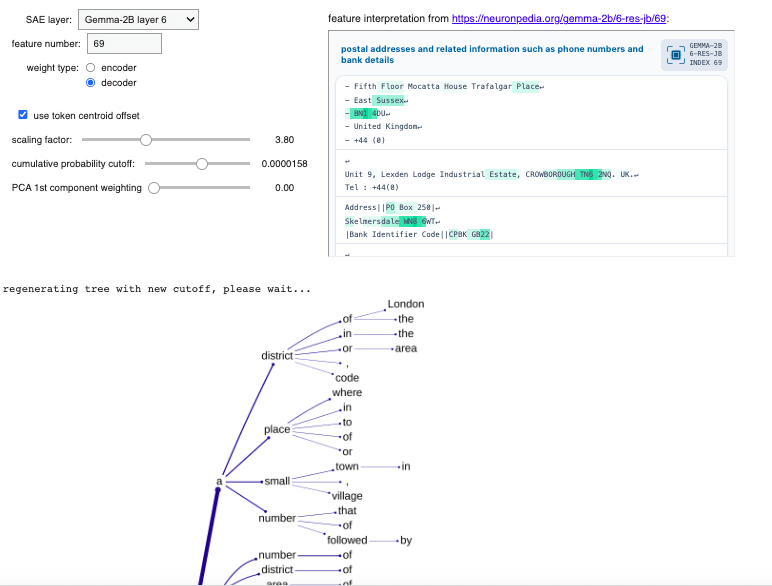
Appendix: Further successful examples

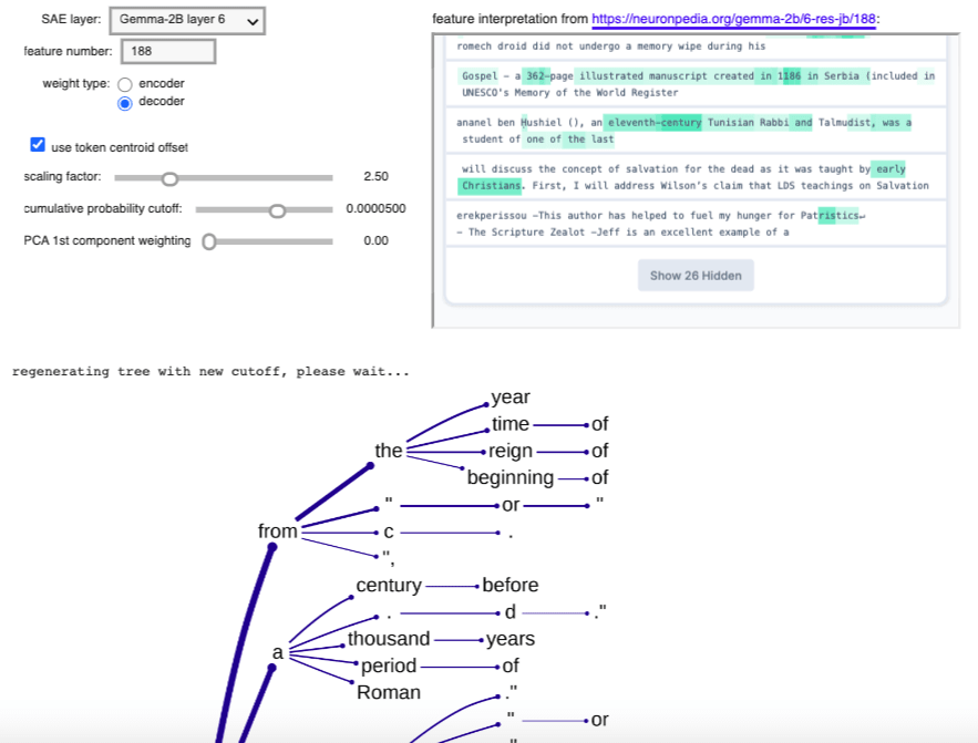
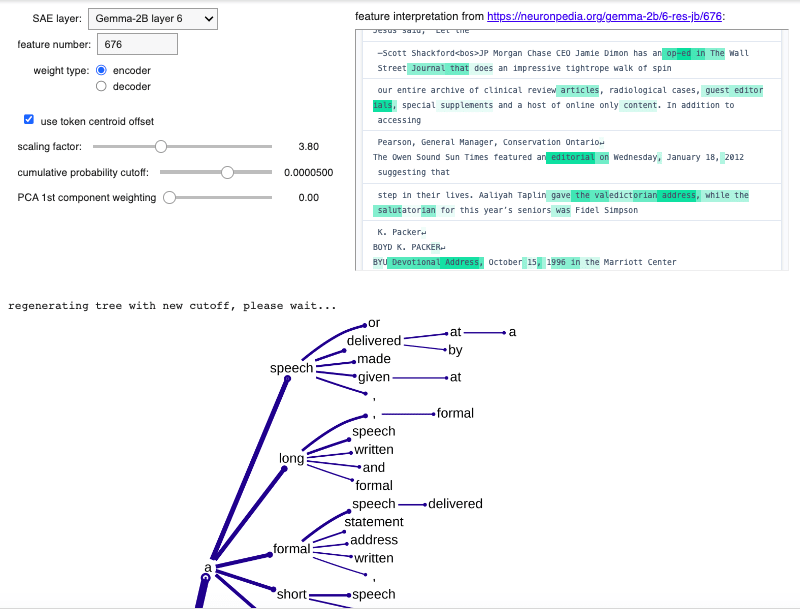
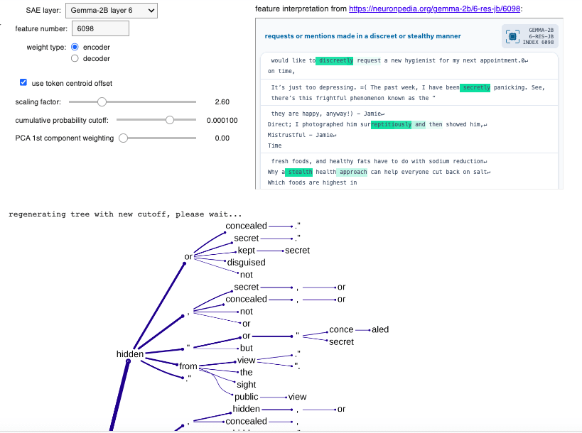
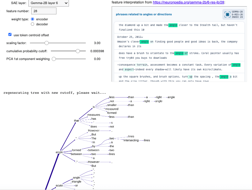
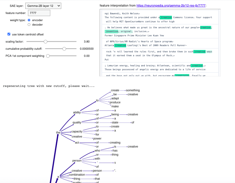
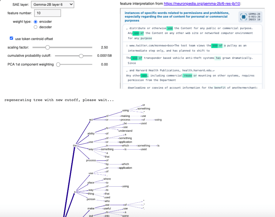
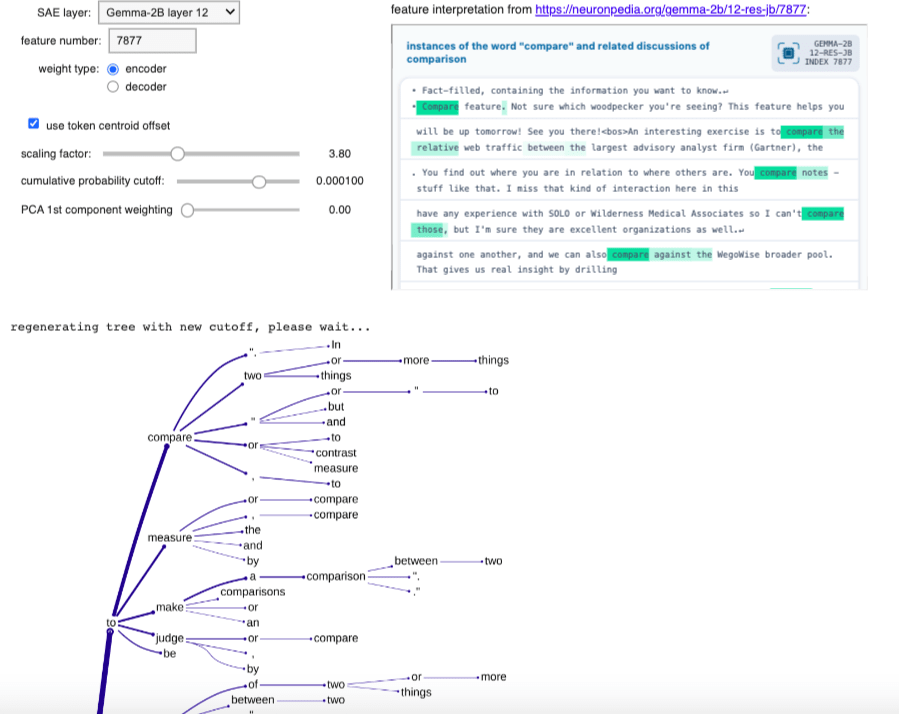
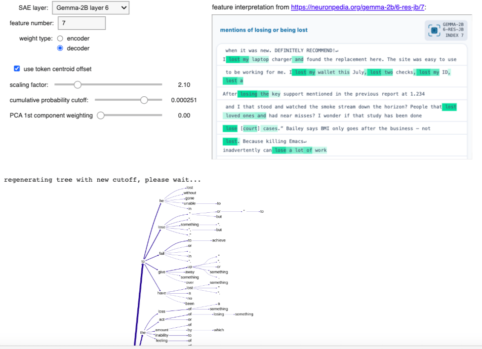
5 comments

Comments sorted by top scores.