Understanding SAE Features with the Logit Lens

post by Joseph Bloom (Jbloom), Johnny Lin (hijohnnylin) · 2024-03-11T00:16:57.429Z · LW · GW · 0 comments

Contents

  Executive Summary
  Introduction
  Characterizing Features via the Logit Weight Distribution
  Token Set Enrichment Analysis
    What is Token Set Enrichment Analysis?
    Method Steps
    Case Studies
        Regex Sets
        NLTK Sets: Starting with a Space, or a Capital Letter
        Arbitrary Sets: Boys Names and Girls Names
  Discussion 
    Limitations
    Future Work
        Research Directions
        More Engineering Flavoured Directions
  Appendix
    Thanks
    How to Cite
    Glossary
    Prior Work 
    Token Set Enrichment Analysis: Inspiration and Technical Details
      Inspiration
      Technical Details
    Results by Layer 
None
No comments

This work was produced as part of the ML Alignment & Theory Scholars Program - Winter 2023-24 Cohort, with support from Neel Nanda and Arthur Conmy. Joseph Bloom is funded by the LTFF, Manifund Regranting Program, donors and LightSpeed Grants. This post makes extensive use of Neuronpedia, a platform for interpretability focusing on accelerating interpretability researchers working with SAEs.

Links: SAEs on HuggingFace, Analysis Code

Executive Summary

This is an informal post sharing statistical methods which can be used to quickly / cheaply better understand Sparse Autoencoder (SAE) features. 

• Firstly, we use statistics (standard deviation, skewness and kurtosis) of the logit weight distributions of features (W_uW_dec[feature]) to characterize classes of features, showing that many features can be understood as promoting / suppressing interpretable classes of tokens. 
  • We propose 3 different kinds of features, analogous to previously characterized “universal neurons”: 
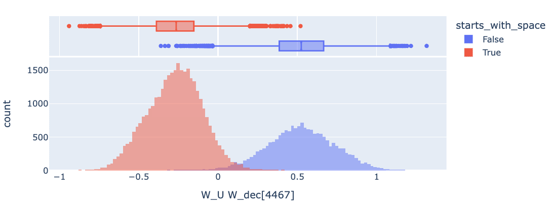
    • Partition Features, which (somewhat) promote half the tokens and suppress the other half according to capitalization and spaces (example pictured below)
    • Suppression Features, which act like partition features but are more asymmetric. 
    • Prediction Features which promote tokens in classes of varying sizes, ranging from promoting tokens that have a close bracket to promoting all present tense verbs. 
• Secondly, we propose a statistical test for whether a feature's output direction is trying to distinguish tokens in some set (eg: “all caps tokens”) from the rest. 
  • We borrowed this technique from systems biology where it is used at scale frequently.
  • The key limitation here is that we need to know in advance which sets of tokens are promoted / inhibited.
• Lastly, we demonstrate the utility of the set-based technique by using it to locate features which enrich token categories of interest (defined by regex formulas, NLTK toolkit parts of speech tagger and common baby names for boys/girls). 
   

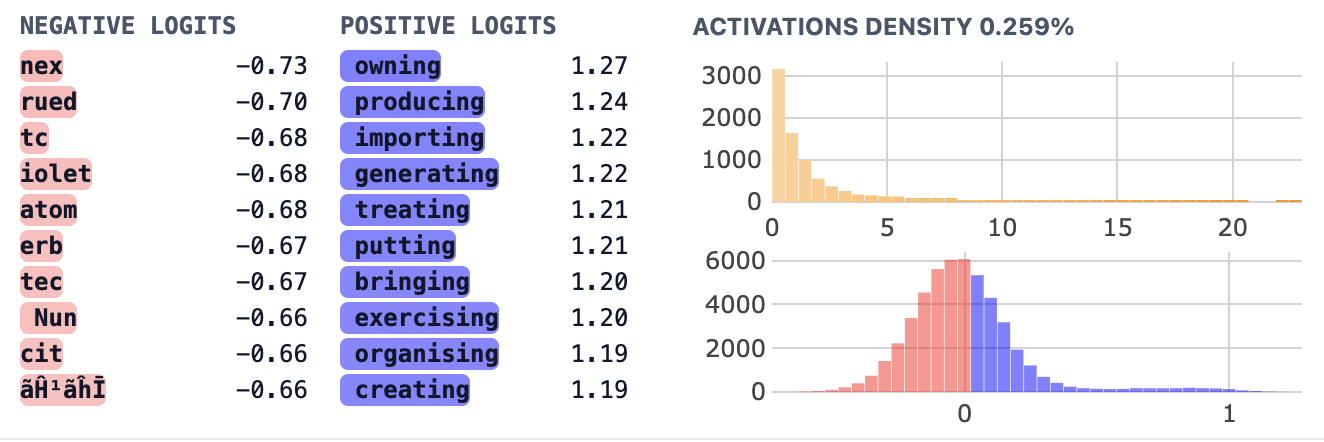
Feature 4467. Above: Feature Dashboard Screenshot from Neuronpedia. It is not immediately obvious from the dashboard what this feature does. Below: Logit Weight distribution classified by whether the token starts with a space, clearly indicating that this feature promotes tokens which lack an initial space character.  

Introduction

In previous work [LW · GW], we trained and open-sourced a set of sparse autoencoders (SAEs) on the residual stream of GPT2 small. In collaboration with Neuronpedia, we’ve produced feature dashboards, auto-interpretability explanations and interfaces for browsing for ~300k+ features. The analysis in this post is performed on features from the layer 8 residual stream of GPT2 small (for no particular reason). 

SAEs might enable us to decompose model internals into interpretable components. Currently, we don’t have a good way to measure interpretability at scale, but we can generate feature dashboards which show things like how often the feature fires, its direct effect on tokens being sampled (the logit weight distribution) and when it fires (see examples of feature dashboards below). Interpreting the logit weight distribution in feature dashboards for multi-layer models is implicitly using Logit Lens [LW · GW], a very popular technique in mechanistic interpretability. Applying the logit lens to features means that we compute the product of a feature direction and the unembed (W_uW_dec[feature]), referred to as the “logit weight distribution”.

 

Since SAEs haven’t been around for very long, we don’t yet know  what the logit weight distributions typically look like for SAE features. Moreover, we find that the form of logit weight distribution can vary greatly. In most cases we see a vaguely normal distribution and some outliers (which often make up an interpretable group of tokens boosted by the feature). However, in other cases we see significant left or right skew, or a second mode. The standard case has been described previously by Anthropic in the context of the Arabic feature they found here and is shown above for feature 6649.

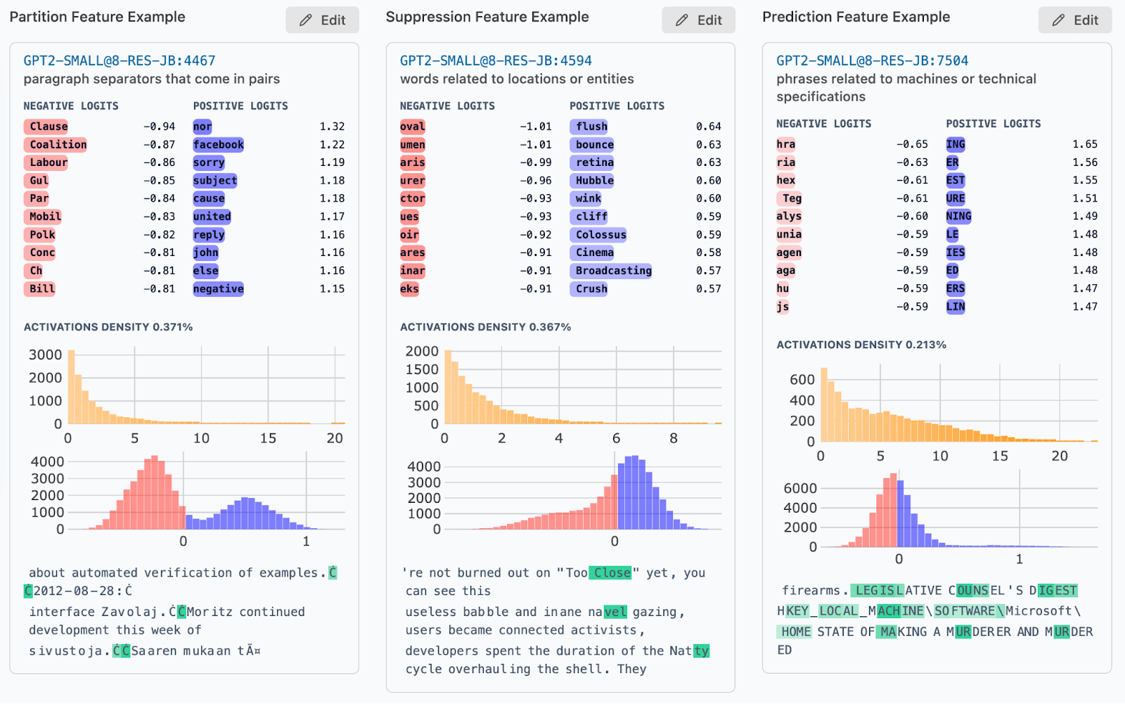
Below, we share some feature dashboard examples which have non-standard characteristics. We refer specifically to the red/blue histogram representing logit weight distribution of each feature, but share other dashboard components for completeness. 

Characterizing Features via the Logit Weight Distribution

To better understand these distributions, (eg: how many have thick tails or how many have lots of tokens shifted left or right), we can use three well known statistical measures:

1. Standard Deviation: Standard deviation measures the spread of a distribution (the average distance of a data point from the mean). 
2. Skewness: Skewness is a measure of how shifted a distribution is. Right-shifted distributions have positive skew and left-shifted distributions have negative skew.
3. Kurtosis: Kurtosis is a measure of the thickness of the tails of a distribution. A kurtosis greater than 3 means a distribution has thicker tails than the normal distribution. 

We note that statistics of the logit weight distribution of neurons have been previously studied in Universal Neurons in GPT2 Language models (Gurnee et al) where universal neurons (neurons firing on similar examples across different models) appeared likely to have elevated W_U kurtosis. Neurons with high kurtosis and positive skew were referred to as “prediction neurons” whilst neurons with high kurtosis and negative skew were described as suppression neurons. Furthermore, partition neurons, which promoted a sizable proportion of tokens while suppressing the remaining tokens, were identifiable via high variance in logit weight distribution. 

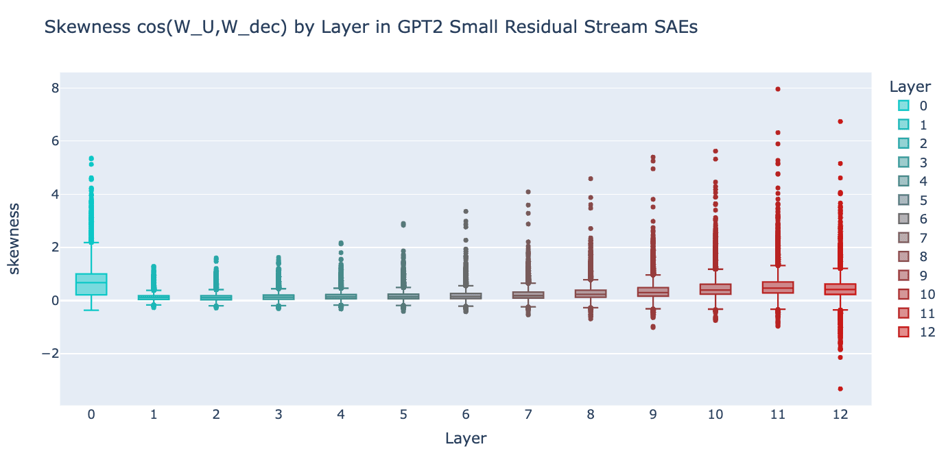
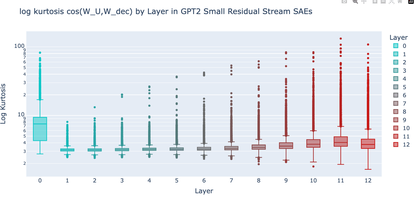
Below, we show a plot of skewness vs kurtosis in the logit weight distribution of each feature, coloring by the standard deviation. See the appendix for skewness / kurtosis boxplots for all layers and this link to download scatterplots for all layers. 

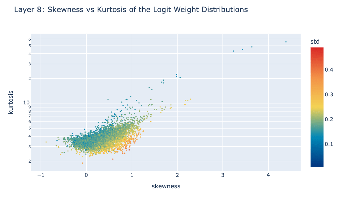
We then use the above plot as a launching point for finding different kinds of features (analogous to types of neurons found by Gurnee et al). 

1. Local Context Features (examples here)
   1. Characterization: Features with high kurtosis. These features are easily identifiable in the top right corner of the plot above.
   2. Interpretation: In general, features with low standard deviation and high kurtosis promote specific tokens or small sets of tokens. The highly noticeable outliers appear to be bracket-closing or quote-closing local context features [LW · GW]. 
2. Partition Features (examples here)
   1. Characterization: These features are identifiable via higher standard deviation (red), right skewness and low kurtosis.
   2. Interpretation: These features have non-standard logit weight distributions, though the “prototypical” features of this class (based on my intuition) are cleanly bimodal. We found it somewhat surprising that the left and right modes correspond to different combinations of whether or not the next token starts with a space and whether or not the next token is capitalized. 
3. Prediction Features (examples here)
   1. Characterization: These features have high skewness and standard deviation that is between 0.03 and 0.07 (yellow/green, but not blue/red). 
   2. Interpretation: These features appear to promote interpretable sets of tokens. There are many different identifiable sets including numerical digits, tokens in all caps and verbs of a particular form. 
4. Suppression Features (examples here)
   1. Characterization: These features have negative skew but low kurtosis, suggesting they might be better understood as suppressing sets of tokens.
   2. Interpretation: I don’t know if there’s a clear boundary between these features and partition features. It seems like they might be partition features (used to reason about a space or capital letter at the start of the next token) which are more context-specific and therefore might suppress a more specific set of tokens.

Token Set Enrichment Analysis

Given previous results, we are particularly interested in identifying the set of tokens which a particular feature promotes or suppresses. Luckily, the field of bioinformatics has been doing set enrichment tests for years and it’s a staple of some types of data analysis in systems biology. We provide some inspiration and technical detail in the appendix, but will otherwise provide only a cursory explanation of the technique.

What is Token Set Enrichment Analysis?

Token Set Enrichment Analysis (TSEA) is a statistical test which maps each logit weight distribution, and a library of sets of tokens, to an “enrichment score” (which indicates how strong that feature seems to be promoting/suppressing each set of features). 

Method Steps

1. Generate a library of token sets. These sets are our “hypotheses” for sets of tokens the model will affect. I expect to develop automated methods for generating them in the future, but for now we use sets that are easy to generate. We assume these sets are meaningful (in fact the test relies on it). 
2. Calculate enrichment scores for all features across all sets. We calculate the running sum statistics which identify which features promote / suppress tokens in the hypothesis sets. In theory, we should calculate p-values by determining distribution of the score under some null hypothesis but we do not think this level of rigor is appropriate at this stage of analysis. 
3. Plot these and look for outliers. The canonical way to represent the results is with a manhattan plot. For our purposes, this is a scatter plot where the x-axis corresponds to features, and the y-axis is -1*log10(enrichment score). Elevated points represent statistically significant results where we have evidence that a particular feature is promoting or suppressing tokens in a particular set. 
4. Inspect features with high enrichment scores. We can then validate “hits” by plotting the distribution of the logit weight by token set membership. This looks like dividing our logit weight distributions into tokens in the enriched set vs not and looking at “outliers” which look like false positives or negatives. 

Case Studies

As a rough first pass, we generate a number of token sets corresponding to:

1. Regex Sets: Sets categorized by regex expressions (eg: starting with a specific letter, or capital, or all digits). Our interpretation of partition features (which distinguish tokens starting with a space or capital letter) can be verified in this way - see the plots at the beginning of the post. 
2. Part-of-Speech Tagging: Sets found by the NLTK part-of-speech tagger. Here we show that various prediction features promote tokens in interpretable sets such as different classes of verbs. 
3. Boy / Girl Names: Here we explore the idea that we can define sets of tokens which correspond to sets we care about, cautiously imposing our own hypothesis about token sets that might be promoted / suppressed in hopes of discovering related prediction features. 

Note: we filter for the top 5000 features by skewness to reduce the over-head when plotting results. 

Regex Sets

Below we show the manhattan plot of the enrichment scores of the top 5000 features by skewness and the following token set:

• Starts with space (33135 tokens). eg: “ token”. 
• Starts with a capital letter (16777 tokens).  eg:  “Token”.
• All digits (1691 tokens). eg: “ 111”. 
• Is punctuation (529 tokens). eg “ )”. 
• Is all capital letters (2775 tokens) - eg: “ TOKEN”. 

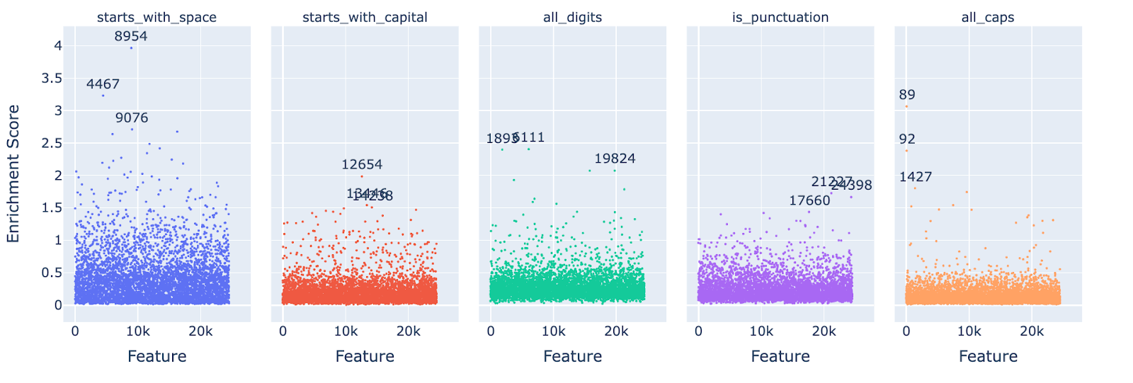
We see that there is a fairly strong token set effect whereby some of the sets we tested achieved generally higher enrichment scores than others. If we wanted to use these results to automatically label features, we’d want to decide on some meaningful threshold here, but let’s first establish we’re measuring what we think we are. 
 

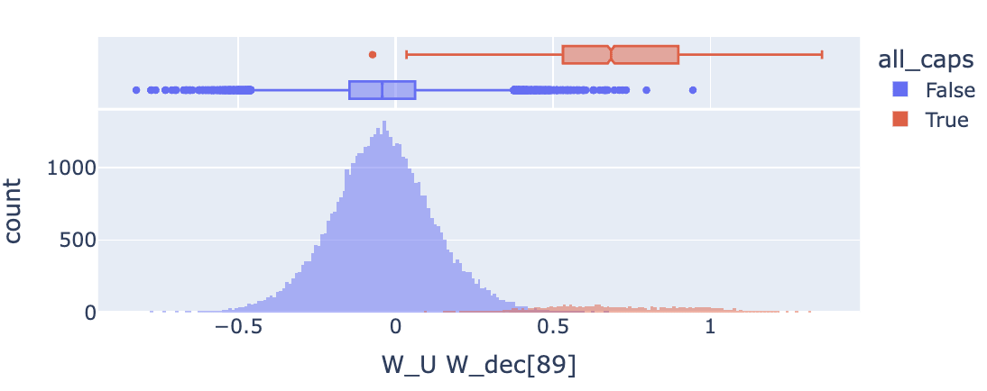
To gain a sense for what kinds of features we show the logit weight distribution for feature 89 below, which was enriched for all caps tokens. We show a screenshot of it’s feature dashboard and a logit weight distribution grouped by the all_caps classification, which show us:

1. The feature dashboard for feature 89 suggested that it promoted 2 capital character tokens beginning with a space. 
2. However, the logit weight distribution histogram makes it appear that many different all caps tokens are directly promoted by this feature. 

Looking at the feature activations on neuronpedia, it seems like the feature is loss reducing prior to tokens that are in all caps but not made only of two tokens, which supports the hypothesis suggested by the TSEA result. 
 

 

NLTK Sets: Starting with a Space, or a Capital Letter

We can use the NLTK part-of-speech tagger to automatically generate sets of tokens which are interesting from an NLP perspective. In practice these sets are highly imperfect as the tagger was not designed to be used on individual words, let alone tokens. We can nevertheless get passable results. 

Let’s go with different types of verbs:

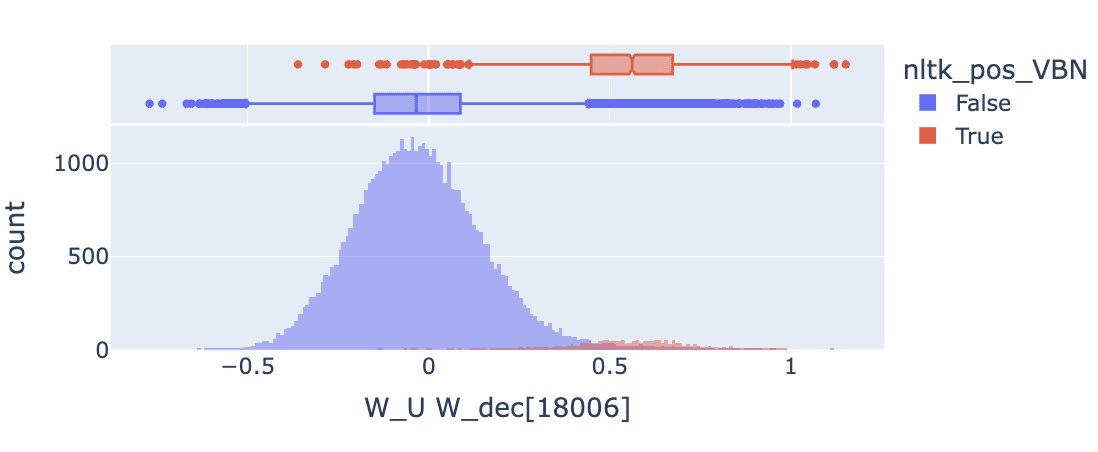
1. VBN: verb, past participle (2007 tokens). Eg: “ astonished”, “ pledged”.  
2. VBG: verb, gerund/present participle taking (1873 tokens).  Eg: “ having”, “ including”. 
3. VB: verb, base form (413 tokens). Eg: “ take”, “ consider”.
4. VBD: verb, past tense took (216 tokens). Eg: “ remained”, “ complained”.
    

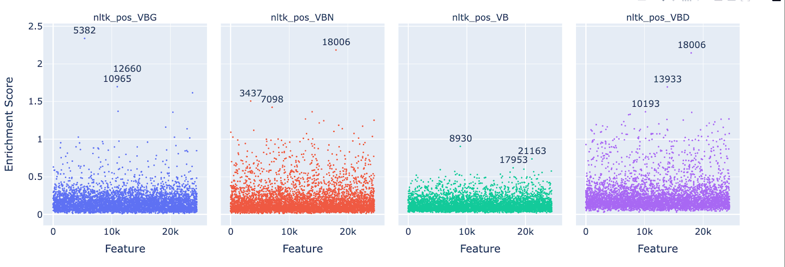
As before, we see a token set effect, though after seeing this result I feel more confident that set size doesn’t explain the set effect.  Why do we not see features for base form verbs achieve higher enrichment scores than other (even smaller) verb sets? Possibly this is an artifact of tokenization in some way, though it's hard to say for sure. As before, let’s look at some examples to gain intuition. 
 

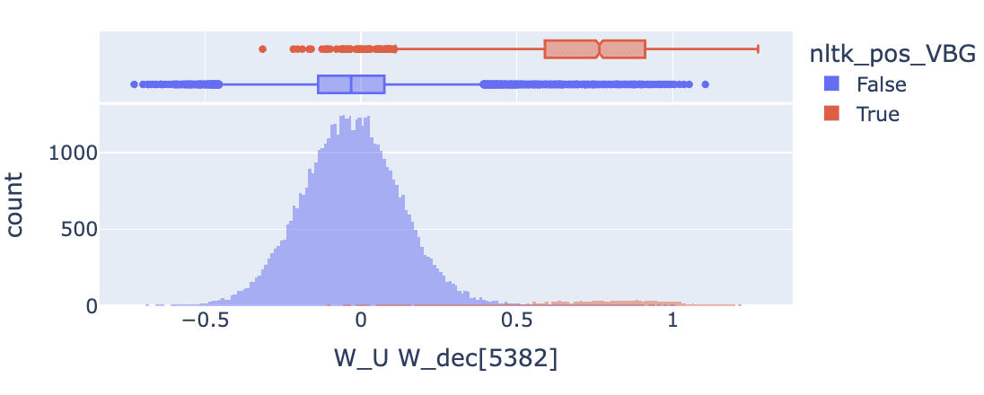
Our largest enrichment score overall is feature 5382 for verbs in the gerund form (ending in ing). I don’t identify a more specific theme in the top 10 positive logits (verbs starting in “ing"), though maybe there is one, so it seems like the enrichment result is in agreement with the statistics. I’m disappointed with the NLTK tagger which said that tokens like “ Viking”, “Ring” and “String” were gerund form verbs (and these are the far left outliers where the feature does not promote those tokens. 

 

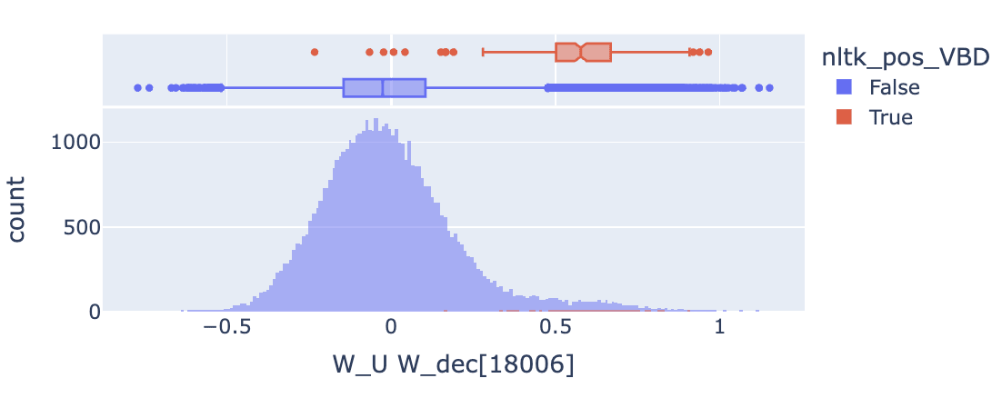
Moving on, feature 18006 appears to promote tokens labeled as past participles (nltk_pos_VBN) as well as past verbs (nltk_pos_VBD). This is actually somewhat expected once you realize that all of these tokens are verbs in the past tense (and that you can’t really distinguish the two out of context). Thus we see that our set enrichment results can be misleading if we aren’t keeping track of the relationship between our sets. To be clear, it is possible that a feature could promote one set and not the other, but to detect this we would need to track tokens which aren’t in the overlap (eg: “began” vs “ begun” or “saw” vs “seen”. I don’t pursue this further here but consider it a cautionary tale and evidence we should be careful about how we generate these token lists in the future. 
 

Arbitrary Sets: Boys Names and Girls Names

Many features in GPT2 small seem fairly sexist so it seemed like an interesting idea to use traditionally gendered names as enrichment sets in order to  find features which promote them jointly or exclusively. Luckily, there’s actually a python package which makes it easy to get the most American first names. We plot the enrichment scores for one set on the x-axis and the enrichment scores for another set on the y-axis to aid us in locating features 

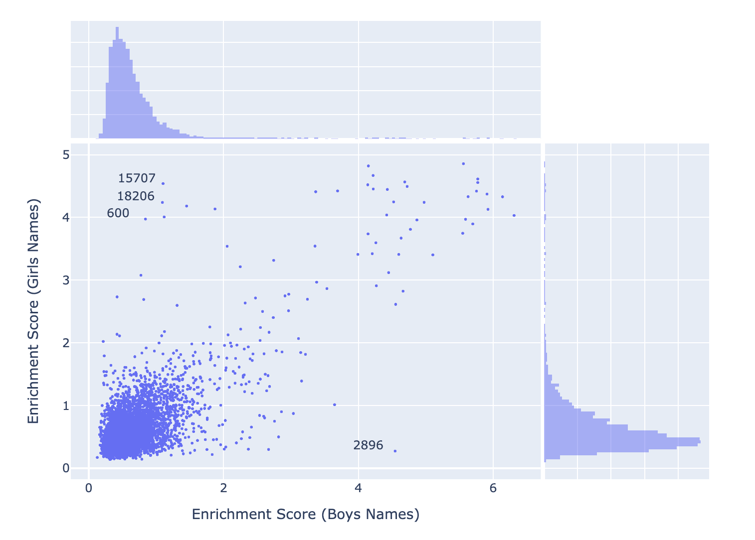
We see here that:

1. Some features score highly for both sets, which we might reasonably understand as name promoting features. 
2. We see more features in the top left corner than the bottom right corner, suggesting that we have some more female name specific features than male specific features. 

To clarify if this has pointed to some interesting features, let’s look at a case study from the bottom right and the top left. 

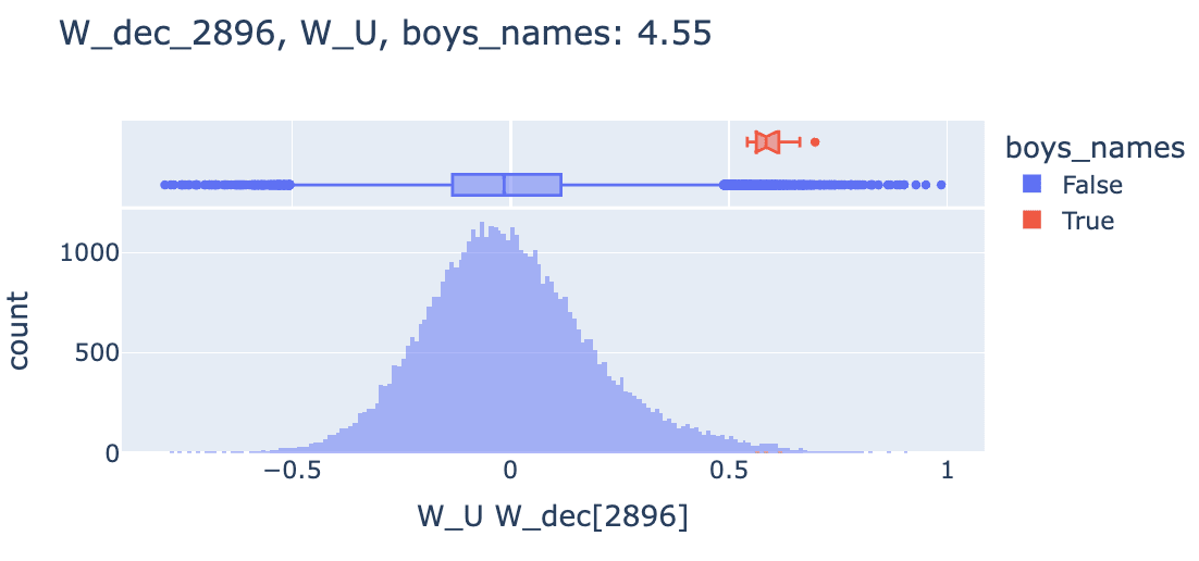
Some observations about Feature 2896:

• On inspection, Feature 2896 does not appear to be a name promoting feature at all, but it does appear to be highly related to gender. Clearly the 300 most common boys names are not the most promoted tokens (via direct effect) but elevated tokens not in the boys_names set include titles like “Mr” and less common boys names. 
• Surprisingly, the top 10 negative logits are very female-oriented. To be clear, it is generally rare for both positive and negative logits to be interpretable, and this is one plausible exception. Moreover, since this feature lacks negative skewness, we wouldn’t have picked up on this as a “suppression feature” though it may genuinely be that it suppresses terms related to women. 
• Looking at max activating examples on neuronpedia, and based on testing out variations on various prompts (eg, this one or this one), I think this feature often fires on punctuation in a prompt after a male pronoun like “he” or “his”. 

Let’s now look at a feature which promoted the girls names over boys names. 

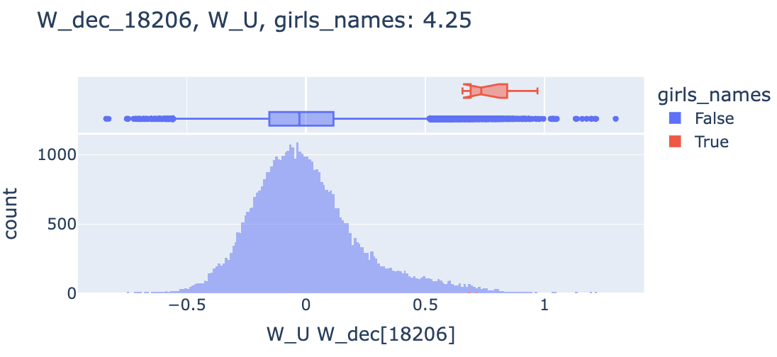
Some observations about feature 18206:

• We see many tokens that are not in the girls_names category which are promoted, but inspection suggests they are girls' names, just not in the top 300, like “ Nicole”, “ Louise” of “Lynn”. I think this suggests that enrichment scores could be stronger if we had better token sets. 
• Looking at max activating examples on neuronpedia, we find that the feature often fires on female names, but fires especially strongly on the second token of a female name that has been split up by tokenization. In this example, the name “Carol” has a variation with a final e - “Carole” which gets tokenized to “ Car” and “ole” and where feature 18206 will fire on the “ole”. The token “ole” on its own won’t make the feature fire, whereas the feature fires on the token “ Carol”.. 
• This is fascinating, though it’s unclear what exactly is happening here  due to the tied embedding of GPT2. It seems more like this is a feature contained in some tokens by default and that something like detokinization [AF · GW]-esque is happening here. 

I think both of these cases studies suggested we had found interesting features that were non-trivially related to boys/names and girls names, but clearly enrichment results can’t be taken at face value due to factors like overlapping sets and the fact we’re apply the logit lens in model with a tied embedding. 

Discussion 

Limitations

I think it’s important to be clear about the limitations of this work so far:

1. I have not quantified the proportion of features which are partition, suppression, prediction or local context features (nor given exact thresholds for how to identify them). Nor have I explored these statistics in detail in other layers or models. 
2. The effect of a feature is not entirely captured by its direct contribution to the logit distribution, so we should be careful not to over-interpret these results. It seems like this might be part of the puzzle, but won’t solve it. Moreover, I’m optimistic that this genre of technique (set enrichment) will help us with these “internal signals” but this is not addressed here.  
3. While it seems likely to me that TSEA over a large number of sets will be cheaper than auto-interp (because of how expensive auto-interp is), it’s definitely not a complete replacement, nor is it clear exactly how expensive or practical it will be to do TSEA at scale.
4. It seems plausible that rather than doing set enrichment over tokens, we should look at it over features. Features are inherently more interpretable and the rich internal structure we really care about is likely between features. Since set enrichment only requires a ranking over objects and a hypothesis set, we can replace tokens with features easily. The current  bottleneck to this is identify which groups of features are meaningful. 

Future Work

Research Directions

• More comprehensively / methodically categorizing features. What proportion of the features are partition features, suppression or prediction features? How many features are straightforwardly not amenable to this kind of analysis? How homogeneous are these features? 
• How misleading might the direct effect of a feature be as compared to its total effect? This whole technique relies on the logit lens which has flaws / can be brittle. It would be good to try to red-team the technique and see if / how it can be misleading. 
• What’s up with features that don’t compose strongly with the unembedding? Can we identify features which are useful for prediction of future tokens rather than the next token? Can we distinguish those from features which are useful for predicting the next token via indirect paths? Can we understand features which are involved in the “dark space”?
• Compile great libraries of token sets. This statistic relies on having predetermined lists of tokens. Regex sets will only get you so far and the NLTK sets aren’t great either.  Obviously it could take a very long time to guess all the sets which should be checked ahead of time, but we have some good alternatives. Some ideas here:
  • Since GPT2-small has a tied embedding, the SAE trained on resid pre 0 finds linear factors in the embedding space which could be useful for defining our sets. For example, see this list of features that correspond to different digit - related groups.
  • Maybe we can use a language model to look through sets of tokens being promoted and manually annotate them. 
• Can we use set enrichment statistics to understand circuits? I suspect that set enrichment can be performed on the residual stream, but that we could also use it as a way to understand circuits. For example, we might use virtual weights by projecting a residual stream feature through the QK and OV circuits and using this to understand the functions of attention heads, using bilinear decompositions with features on one side and tokens on the other. 
• Can we use logit distribution statistics as proxies for interpretability to help us better understand what is happening during training of SAEs? Training SAEs is hard in part because we lack good proxies for interpretability. To the degree that it seems like some aspects of interpretability may be captured fairly easily by statistics of the logit weight distribution, this may inform our understanding of what is happening during training or what effects changes in hyperparameters (such as the l1 coefficient) have on our results. 
• Anti-Direction: I don’t think I would be particularly excited about working very hard to get very significant results with the TSEA statistic, due to similar perspectives expressed in this recent post. I think the case studies I showed above speak to lots of different kinds of messiness that we should try to understand and or deal with directly. 

More Engineering Flavoured Directions

• Using TSEA in practice: The recipe for this will look like:
  • Compile a long list of sets which you want to perform TSEA over. 
  • For each feature, test each hypothesis (estimating the FDR associated with doing however many tests are done in total to avoid p-hacking). 
  • Present significant results alongside feature dashboards or make them directly browseable. 
  • Optionally: Provide these results to model performing automatic interpretability. 
• Can we make a tuned-lens version of this technique?
• Find a way to leverage highly optimized GSEA software to quickly make the technique more scalable.
• Explore how much set enrichment results can improve automatic interpretability. 

Appendix

Thanks

I’d like to thank Neel Nanda and Arthur Conmy for their support and feedback while I’ve been working on this and other SAE related work. 

I’d like to thank Johnny Lin for his work on Neuronpedia and ongoing collaboration which makes working with SAEs significantly more feasible (and enjoyable!). 

I also appreciate feedback and support from Andy Arditi. Egg Syntax, Evan Anders and McKenna Fitzgerald.

How to Cite

@misc{bloom2024understandingfeatureslogitlens,
   title = {Understanding SAE Features with the Logit Lens},
   author = {Joseph Bloom, Johnny Lin},
   year = {2024},
   howpublished = {\url{https://www.lesswrong.com/posts/qykrYY6rXXM7EEs8Q/understanding-sae-features-with-the-logit-lens}},
}

 

Glossary

• W_dec . The decoder weights of a sparse autoencoder. 
• W_U. The Unembedding Matrix of a Transformer. 
• W_uW_dec[feature]. The logit weight distribution. A projection of the residual stream onto the token space. 
• GSEA: Gene Set Enrichment Analysis. A technique for checking whether proteins in a predefined set are elevated in a ranking (such as expression in cancer cells over healthy cells). 
• TSEA: GSEA, but applied to the logit weight distribution and sets of tokens rather than genes / proteins. (see appendix). 

Prior Work 

• Logit Lens: interpreting GPT: the logit lens — LessWrong [LW · GW] 
• Classifying Neurons / Features: [2401.12181] Universal Neurons in GPT2 Language Models 
• SAEs
  • Recent Papers
    • [2309.08600]  Sparse Autoencoders Find Highly Interpretable Features in Language Models 
    • Towards Monosemanticity: Decomposing Language Models With Dictionary Learning
  • Update:
    • Circuits Updates - January 2024 
  • Replications
    • Open Source Replication & Commentary on Anthropic's Dictionary Learning Paper — LessWrong [LW · GW]
    • Some open-source dictionaries and dictionary learning infrastructure — AI Alignment Forum [LW · GW] 
    • https://github.com/openai/sparse_autoencoder
  • Advice:
    • My best guess at the important tricks for training 1L SAEs — LessWrong [LW · GW] 
    • Some additional SAE thoughts — LessWrong [LW · GW] 
  • Nanda MATS Stream results
    • Case Studies in Reverse-Engineering Sparse Autoencoder Features by Using MLP Linearization — LessWrong [LW · GW] 
    • Sparse Autoencoders Work on Attention Layer Outputs — LessWrong [LW · GW]
    • We Inspected Every Head In GPT-2 Small using SAEs So You Don’t Have To — LessWrong [LW · GW] 

 

Token Set Enrichment Analysis: Inspiration and Technical Details

Inspiration

Gene Set Enrichment Analysis (GSEA) is a statistical method used to check if the genes within some set are elevated within some context. Biologists have compiled extensive sets of proteins associated with different biological phenomena which are often used as a reference point for various analyses. For example, the Gene Ontology Database contains hierarchical sets which group proteins by their structures, processes and functions. Other databases group proteins by their interactions or involvement in pathways (essentially circuits). Each of these databases support GSEA, which is routinely used to map between elevated levels of proteins in samples and broader knowledge about biology or disease. For example, researchers might find that the set of proteins associated with insulin signally are in particularly low abundance in patients with type 2 diabetes, indicating that insulin signaling may be related to diabetes. 

 

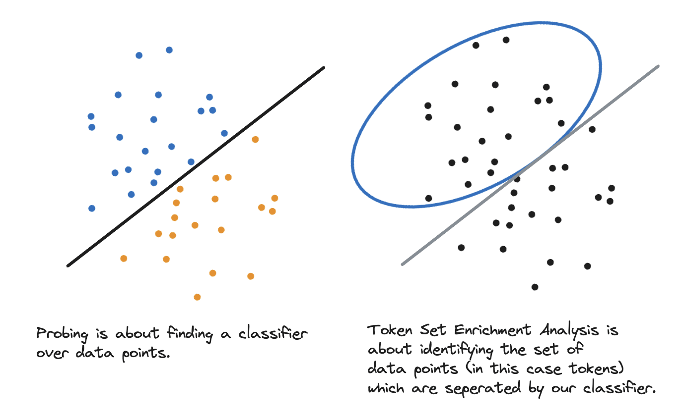
Here, we’re going to perform Token Set Enrichment Analysis, which you can think of as a kind of “reverse probing”. When probing, we train a classifier to distinguish data points according to some labels. Here, SAEs have already given us a number of classifiers (over tokens) and we wish to know which sets of tokens they mean to distinguish. The solution is to use a cheap statistical test which takes a hypothesis set of tokens, and checks whether they are elevated in the logit weight distributions. 

Technical Details

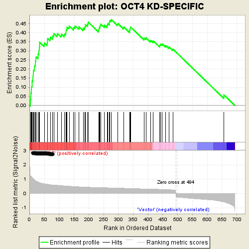
If we treat each of our feature logit distributions as a ranking over tokens, and then construct sets of interpretable tokens, we can calculate a running-sum statistic which quantifies the elevation of those tokens in each of the logit weight distributions for each set. The score is calculated by walking down the logit weight distribution, increasing a running-sum statistic when we encounter a token in the set, S, and decreasing it when we encounter a token not in S.
 

The figure below is a standard GSEA “enrichment plot” showing the running sum statistic for some set / ranking over genes. We note that usually a false discovery rate is estimated when performing large numbers of these tests. We’ve skipped this procedure as we’re short on time, but this should be implemented when this technique is applied at scale. 
 

Results by Layer 

See this file for scatter plots for skewness and kurtosis for each layer. 


 

0 comments

Comments sorted by top scores.