Attention Output SAEs Improve Circuit Analysis

post by Connor Kissane (ckkissane), robertzk (Technoguyrob), Arthur Conmy (arthur-conmy), Neel Nanda (neel-nanda-1) · 2024-06-21T12:56:07.969Z · LW · GW · 0 comments

Contents

  Executive Summary
  Introduction
  Evaluating our SAEs for IOI Circuit Analysis
  Case Study: Applying SAEs for Deeper Understanding of IOI 
    Identifying the Positional Features with SAEs
    Interpreting the “Positional” Features
    Confirming the Hypothesis 
    Applying SAEs to QK circuits: S-Inhibition Heads Sometimes Do IO-Boosting
  Discovering Attention Feature Circuits with Recursive DFA
    Understanding Recursive DFA
    Example: Attention feature 3.15566 decomposes into gender and name information
    Example: Retrieving "Dave" using recursive attention attribution.
    Even Cooler Examples: Win a $1000 Bounty!
  Related Work
  Conclusion
    Limitations
    Future Work
  Citing this work
  Author Contributions Statement
None
No comments

This is the final post of our Alignment Forum sequence produced as part of the ML Alignment & Theory Scholars Program - Winter 2023-24 Cohort.

Executive Summary

• In a previous post we trained Attention Output Sparse Autoencoders (SAEs) [LW · GW] on every layer of GPT-2 Small [LW · GW]. 
• Following that work, we wanted to stress-test that Attention SAEs were genuinely helpful for circuit analysis research. This would both validate SAEs as a useful tool for mechanistic interpretability researchers, and provide evidence that they are identifying the real variables of the model’s computation.
• We believe that we now have evidence that attention SAEs can:
  • Help make novel mechanistic interpretability discoveries that prior methods could not make.
  • Allow for tracing information through the model’s forward passes on arbitrary prompts.
• In this post we discuss the three outputs from this circuit analysis work:

1. We use SAEs to deepen our understanding of the IOI circuit. It was previously thought that the indirect object’s name was identified by tracking the names positions, whereas we find that instead the model tracks whether names are before or after “and”. This was not noticed in prior work, but is obvious with the aid of SAEs.
2. We introduce “recursive direct feature attribution” (recursive DFA) and release an Attention Circuit Explorer tool for circuit analysis on GPT-2 Small (Demo 1 and Demo 2). One of the nice aspects of attention is that attention heads are linear when freezing the appropriate attention patterns. As a result, we can identify which source tokens triggered the firing of a feature. We can perform this recursively to track backwards through both attention and residual stream SAE features in models.
   1. We also announce a $1,000 bounty for whomever can produce the most interesting example of an attention feature circuit by 07/15/24 as subjectively assessed by the authors. See the section "Even cooler examples" for more details on the bounty.
3. We open source HookedSAETransformer to SAELens, which makes it easy to splice in SAEs during a forward pass and cache + intervene on SAE features. Get started with this demo notebook.

Introduction

With continued investment into dictionary learning research, there still remains a concerning lack of evidence that SAEs are useful interpretability tools in practice. Further, while SAEs clearly find interpretable features (Cunningham et al.; Bricken et al.), it's not obvious that these features are true causal variables used by the model. In this post we address these concerns by applying our GPT-2 Small Attention SAEs [LW · GW] to improve circuit analysis research.

We start by using our SAEs to deepen our understanding of the IOI task. The first step is evaluating if our SAEs are sufficient for the task. We “splice in” our SAEs at each layer, replacing attention layer outputs with their SAE reconstructed activations, and study how this affects the model’s ability to perform the task - if crucial information is lost by the SAE, then they will be a poor tool for analysis. At their best, we find that SAEs at the early-middle layers almost fully recover model performance, allowing us to leverage these to answer a long standing open question and discover novel insights about IOI. However, we also find that our SAEs at the later layers (and layer 0) damage the model's ability to perform the task, suggesting we’ll need more progress in the science and scaling of SAEs before we can analyze a full end-to-end feature circuit.

We then move beyond IOI and develop a visualization tool (link) to explore attention feature circuits on arbitrary prompts, introducing a new technique called recursive DFA. This technique exploits the fact that transformers are almost linear if we freeze attention patterns and LayerNorm scales, allowing us to compute the direct effect of upstream features in computing downstream features. This also allows us to mostly sidestep more expensive (and arguably less principled) causal intervention techniques. 

Overall, we found that SAEs were a valuable tool that gave us novel insights into circuits that had already been studied manually in a lot of detail. However, they were unreliable and far from a silver bullet, with several layers having significant reconstruction error. Significant further work needs to be done before they can be a reliable tool to analyze arbitrary circuits, and we recommend that practitioners begin any circuit analysis by carefully checking for whether the SAE destroys key info. 

Evaluating our SAEs for IOI Circuit Analysis

Currently SAEs are evaluated by proxy metrics such as the average number of features firing (L0 norm) and average cross entropy loss recovered. However we’d ultimately like to use SAEs for concrete interpretability questions. As a case study, we wanted to determine whether SAEs provided a story consistent with our understanding of the IOI task (Wang et al.), or even deepened it. SAEs inherently introduce some reconstruction error, so the first step was to check whether SAEs preserved the model’s ability to perform IOI.

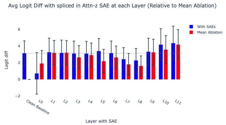
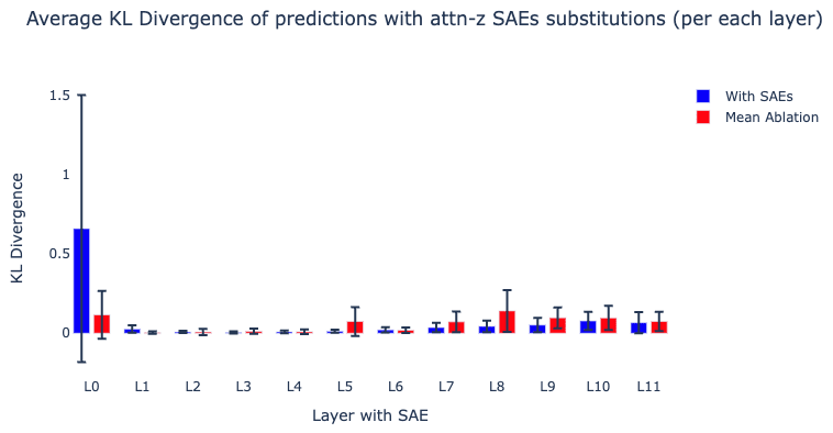
For each layer, we replace attention output activations with their SAE reconstructed activations and observe the effect on the average logit difference between the correct and incorrect name tokens (as in Makelov et al.). We also measure the KL divergence between the logits of the original model and the logits of the model with the SAE attached. We also compare the effect of splicing in the SAEs to mean ablating these attention layer outputs from the ABC distribution [LW · GW] (“Then, [A] and [B] went to the [PLACE]. [C] gave an [OBJECT] to”) to also get a rough sense of how necessary these activations are for the circuit. 

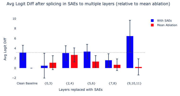
We find that splicing in our SAEs at each of the early-middle layers [1, 6] maintains an average logit difference roughly equal to the clean baseline, suggesting that these SAEs are sufficient for circuit analysis. On the other hand, we see layers {0, 7, 8} cause a notable drop in logit difference. The later layers actually cause an increase in logit difference, but we think that these are likely breaking things based on the relatively high average KL divergence, illustrating the importance of using multiple metrics that capture different things.^[1]

The IOI paper identifies many classes of attention heads (e.g. duplicate token heads) spread across multiple layers. To investigate if our SAEs are systematically failing to capture certain feature families, we splice in our SAEs for each of these cross-sections (similar to Makelov et al.)

For each role classified in the IOI paper, we identify the set of attention layers containing all of these heads. We then replace the attention output activations for all of these layers with their reconstructed activations. Note that we recompute the reconstructed activations sequentially rather than patching all of them in at once. We do this for the following groups of heads identified in the paper:

• Duplicate token Heads {0, 3}
• Previous token heads {2, 4}
• Induction heads {5, 6}
• S-inhibition heads {7, 8}
• (Negative) Name Mover Heads {9, 10, 11}

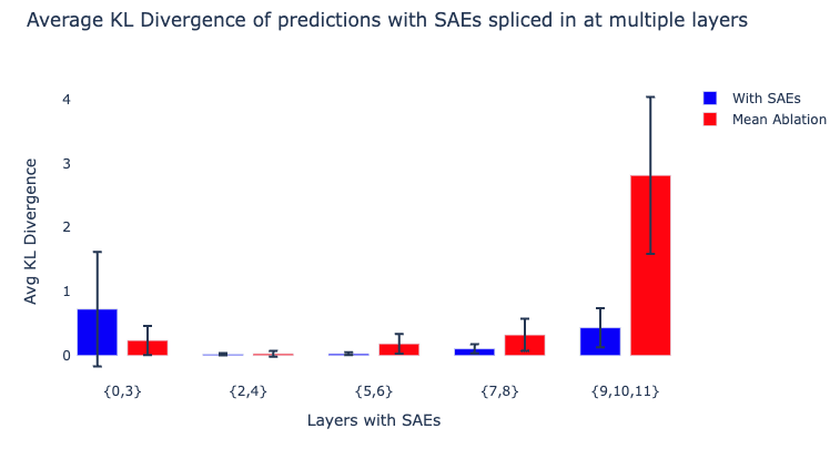
We again see promising signs that the early-middle layer SAEs (corresponding to the induction and previous token heads) seem sufficient for analysis at the feature level. Unfortunately, it’s also clear that our SAEs are likely not sufficient to analyze the outputs of the later layers (S-inhibition heads and (Negative) Name Movers) and Layer 0. Thus we are unable to study a full end-to-end feature circuit for IOI.

Why is there such a big difference between cross-sections? We don’t know, but hypothesize that the middle layers contain more general features like “I am a duplicate token [AF · GW]”, while the late layers contain niche name specific features like “The name X is next [AF · GW]”. Not only do we expect much more per-name features, but we also expect these features to be relatively rare, and thus harder for the SAEs to learn during training. We hope that this will be improved by ongoing work on science and scaling of SAEs (Rajamanoharan et al.; Templeton et al.).

Case Study: Applying SAEs for Deeper Understanding of IOI 

We now leverage some of our better SAEs to study the IOI circuit. The Indirect Object Identification (IOI) task (Wang et al.) is to complete sentences like “After John and Mary went to the store, John gave a bottle of milk to” with “ Mary'' rather than “ John”. We refer to the repeated name (John) as S (the subject) and the non-repeated name (Mary) as IO (the indirect object). For each choice of the IO and S names, there are two prompt templates: one where the IO name comes first (the 'ABBA' template) and one where it comes second (the 'BABA' template).

The original IOI paper argues that GPT-2 Small solves this task via the following algorithm:

1. Induction Heads and Duplicate token heads identify that S is duplicated. They write information to the S2 residual stream that indicates that this token is duplicated, as well as “positional signal” pointing to the S1 token.
2. S-inhibition heads route this information from S2 to END via V-composition. They output both token and positional signals that cause the Name mover heads to attend less to S1 (and thus more to IO) via Q-composition.
3. Name mover heads attend strongly to the IO position and copy, boosting the logits of the IO token that they attend to.

Although Wang et al. find that “positional signal” originating from the induction heads is a key aspect of this circuit, they don’t figure out the specifics of what this signal is,
and ultimately leave this mystery as one of the “most interesting future directions” of their work. Attention Output SAEs immediately reveal the positional signal through the feature lens. We find that rather than absolute or relative position between S tokens, the positional signal is actually whether the duplicate name comes after the “ and” token that connects “John and Mary”.

Identifying the Positional Features with SAEs

To investigate the positional signal encoded in the induction layer outputs, we use our Attention SAEs to decompose these outputs into a linear combination of interpretable SAE features plus an error term (as in Marks et al.). For now we focus on our Layer 5 SAE, one of the layers with induction heads. 

Our initial goal is to identify causally relevant features. We do this by zero ablating each feature one at a time and recording the resulting change in logit difference. Despite there being hundreds of features that fire at this position at least once over 100 prompts, zero ablations narrow down three features that cause an average decrease in logit diff greater than 0.2. Note that ablating the error term has a minor effect relative to these features, corroborating our evaluations that our L5 SAE is sufficient for circuit analysis. We distinguish between ABBA and BABA prompts, as we find that the model uses different features based on the template. 

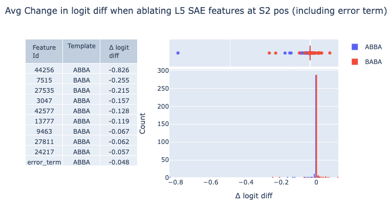
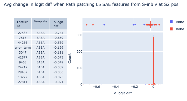
We also localize the same three features when path patching features out of the S-inhibition head values, suggesting that these features are meaningfully V-composing with these heads, as the IOI paper would suggest.

Interpreting the “Positional” Features

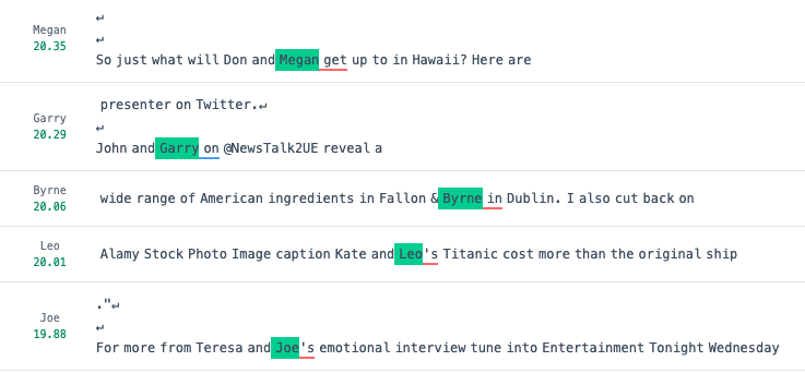
We find that features L5.F7515 and L5.F27535 are the most important for the BABA prompts, while feature L5.F44256 stands out for ABBA prompts. Shallow investigations suggest that all three of these fire on duplicate tokens, and all have some dependence on prior “ and” tokens. We hypothesize that the two BABA features are variants of “I am a duplicate token that previously preceded ‘ and’” features, while the ABBA feature is “I am a duplicate token that previously followed ‘ and’”. Note we additionally find similar causally relevant features from the induction head in Layer 6 and the duplicate token head in layer 3 (see appendix).
 

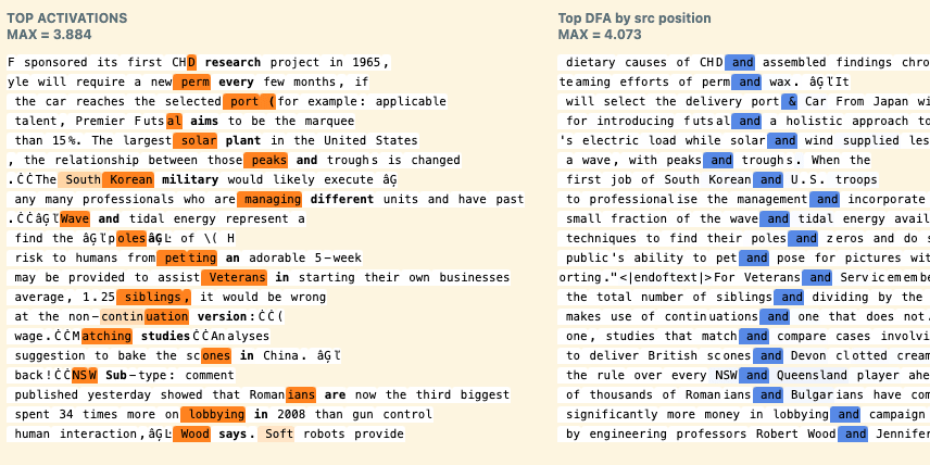
As an interesting aside, our head attribution technique [AF · GW] suggests that all three of these features primarily come from an induction head (5.5) output. Notably, it would be extremely hard to distinguish the differences between these features without SAEs, as the induction head’s attention pattern would just suggest the head is “doing induction” in both cases. This is further evidence that circuit analysis at the level of heads might be too coarse grained and can be misleading, validating the usefulness of Attention SAE features as potentially better units of analysis. We give additional thoughts in the appendix.

Confirming the Hypothesis 

The features motivate the hypothesis that the “positional signal” in IOI is solely determined by the position of the name relative to (i.e. before or after) the ‘ and’ token. This is a bold claim, but we now verify this hypothesis without reference to SAEs. We design a noising (defined by Heimersheim and Nanda) experiment that perturbs three properties of IOI prompts simultaneously, while preserving whether the duplicate name is before or after the ‘ and’ token. Concretely, our counterfactual distribution makes the following changes:

• Replacing each name with another random name (removing token signal)
• Prepend filler text (corrupting absolute positions) 
• Add more filler text between S1 and S2 (corrupting the relative position), 

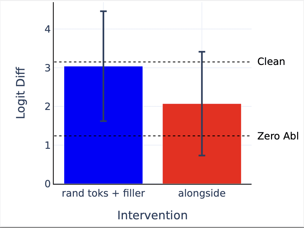
Despite being almost entirely different prompts, noising the attention layer outputs for both induction layers [5, 6] at the S2 position still recovers ~93% of average logit diff relative to zero ablating the outputs at this position.

One alternate hypothesis is that the positional signal is a more general emergent positional embedding [AF · GW] (e.g. “I am the second name in the sentence”) that doesn’t actually depend on the “ and” token. We falsify this by nosing attn_out at layers [5,6] S2 position from a corrupted distribution which only changes “ and” to the token “ alongside”. Note that this only corrupts one piece of information (the ‘ and’) compared to the three corruptions above, yet we only recover ~43% of logit diff relative to zero ablation.^[2]

Applying SAEs to QK circuits: S-Inhibition Heads Sometimes Do IO-Boosting

In addition to answering an open question about the positional signal in IOI, we also can use our SAEs to learn new mechanisms for how these positional features are used downstream. Recall that Wang et al. found that the induction head outputs V-compose with the S-inhibition heads, which then Q-compose with the Name Mover heads, causing them to attend to the correct name. Our SAEs allow us to zoom in on this sub-circuit in finer detail.

We use the classic path expansion trick from A Mathematical Framework for Transformer Circuits to zoom in on a Name Mover head’s QK sub-circuit for this path:^[3]

$${\text{x}}_{\text{attn}}{W}_{OV}^{\text{S-inb}}{W}_{QK}^{NM}({\text{x}}_{\text{resid}}{)}^{⊺}$$

Where ${\text{x}}_{\text{attn}}$ is the attention output for a layer with induction heads, $W_{OV}^{\text{S-inb}}$ is the OV matrix for an S-inhibition head, $W_{QK}^{NM}$ is the QK matrix for a name mover head, and ${\text{x}}_{\text{resid}}$ is the residual stream which is the input into the name mover head. For this case study we zoom into induction layer 5, S-inhibition head 8.6, and Name Mover head 9.9. 

While the ${\text{x}}_{\text{attn}}$ and ${\text{x}}_{\text{resid}}$ terms on each side are not inherently interpretable units (e.g. the residual stream is tracking a large number of concepts at the same time, cf the superposition hypothesis), SAEs allow us to rewrite these activations as a weighted sum of sparse, interpretable features plus an error term. For an arbitrary activation $\text{x}$ that we reconstruct with an SAE, we can write (using similar notation to Marks et al.):

$$\text{x}=\hat{\text{x}}+ϵ\left(\text{x}\right)=\sum _{i=0}^{d_{\text{sae}}}{f}_i\left(\text{x}\right){\text{d}}_i+\text{b}+ϵ\left(\text{x}\right)$$

Where x is the SAE reconstruction, $ϵ\left(\text{x}\right)$ is the SAE “error term”, $f_i\left(\text{x}\right)$ are SAE feature activations, ${\text{d}}_i$ are the SAE decoder feature directions, and $\text{b}$ is the SAE decoder bias. 

This allows us to substitute both the ${\text{x}}_{attn}$ and ${\text{x}}_{resid}$ (using Joseph Bloom’s resid_pre SAEs [LW · GW]) terms with their SAE decompositions.^[4] We then multiply these matrices to obtain an interpretable look up table between SAE features for this QK sub-circuit: Given that this S-inhibition head moves some layer 5 attn SAE feature to be used as a Name Mover query, how much does it “want” to attend to a residual stream feature on the key side. 

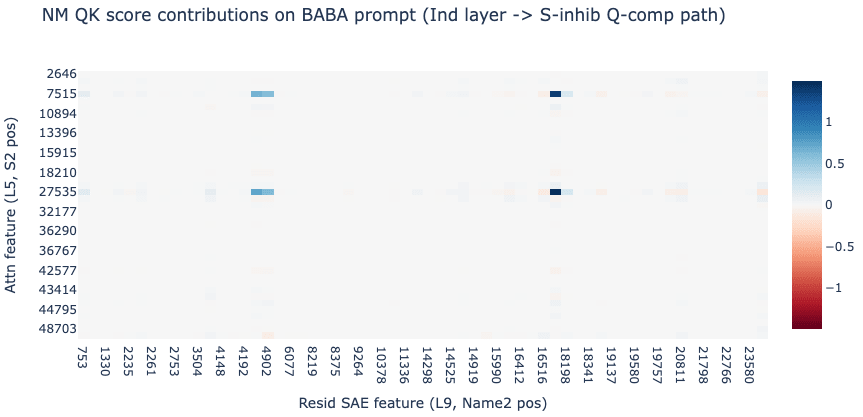
Fascinatingly, we find that the attention scores for this path can be explained by just a handful of sparse, interpretable pairs of SAE features. We zoom into the attention score from the END destination position to the Name2 source position^[5] (e.g. ‘ Mary’ in “ When John and Mary …”).

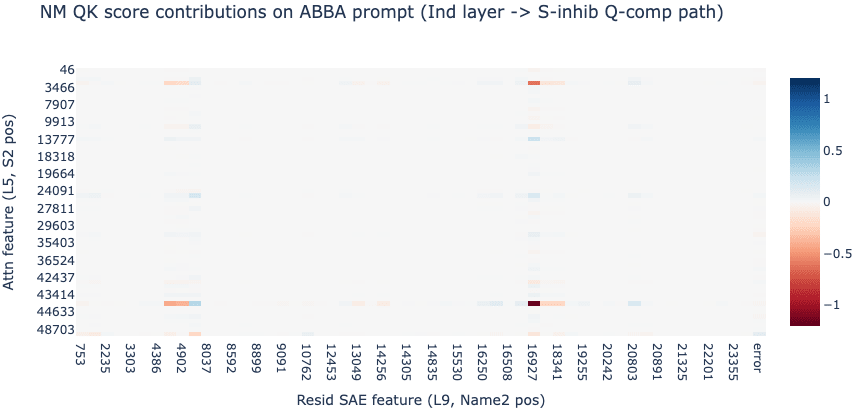
We observe that these heat maps are almost entirely explained by a handful of common SAE features. On the query side we see the same causally relevant Attention SAE features previously identified by ablations: L5.7515 and L5.27535 (“I am a duplicate that preceded ‘ and’”) for BABA prompts while ABBA prompts show L5.44256 and L5.3047 (“I am a duplicate that followed ‘ and’”). On the key side we also find just 2 common residual stream features doing most of the heavy lifting: L9.16927 and L9.4444 seem to activate on names following “ and”.

We also observe a stark difference in the heatmaps between prompt templates: while these pairs of features cause a decrease in attention score on the ABBA prompts, we actually see an increase in attention score on the BABA prompts. This suggests a slightly different algorithm between the two templates. On ABBA prompts, the S-inhibition heads move “I am a duplicate following ‘and’” to “don’t attend to the name following ‘ and’” (i.e. S-inhibition), while in BABA prompts it moves “I am a duplicate before ‘ and’” to “attend to the name following and”. This suggests that the S-inhibition heads are partially doing “IO-boosting” on these BABA prompts. 

To sanity check that our SAE based interpretations are capturing something real about this QK circuit, we compute how much of the variance in these heat maps is explained by just these 8 pairs of interpretable SAE features.^[6] We find that these 8 pairs of SAE features explain 62% of the variance of the scores over all 100 prompts. For reference, all of the entries that include at least one error term (for both the attn and resid SAEs) only explain ~15% of the variance:

${\sum }_{i=0}^{d_{\text{sae}}^{\text{resid}}}\epsilon \left(x_{\text{attn}}\right)W_{OV}^{\text{S-inb}}f\left(x_{\text{resid}}\right)v_i^{\text{resid}}+{\sum }_{j=0}^{d_{\text{sae}}^{\text{attn}}}f\left(x_{\text{attn}}\right)v_j^{\text{attn}}{W}_{OV}^{\text{S-inb}}\epsilon \left(x_{\text{resid}}\right)+\epsilon \left(x_{\text{attn}}\right)W_{OV}^{\text{S-inb}}\epsilon \left(x_{\text{resid}}\right)$

Discovering Attention Feature Circuits with Recursive DFA

As argued in our initial post [AF · GW], each feature activation is a sum of contributions from each head. We call the decomposition into per-head scores direct feature attribution (DFA). 

We can extend the DFA technique by taking advantage of the fact that once attention patterns and layer norm scales have been frozen, there is a linear contribution from i) different token position residual streams, ii) upstream model components, and iii) upstream attention SAE decoder weight features to downstream attention SAE features. This allows for a much more fine-grained decomposition and as we run into attention SAE features upstream we can perform this recursively. 

We release a tool (link) that enables performing this kind of recursive DFA (RDFA) on arbitrary prompts for GPT-2 Small. We currently only support this recursive attribution from attention to attention components, as we cannot pass upstream linearly through MLPs. See the Future Work section for discussion of ways to work around this limitation, such as the use of MLP transcoders [AF · GW].

Understanding Recursive DFA

At a high level, the idea of RDFA is that so long as the contribution of MLPs to a given behavior is not that significant, we can use Attention SAEs [AF · GW] and residual stream SAEs [AF · GW] to repeatedly attribute SAE feature activation to upstream SAE feature outputs, all the way back to the input tokens. Here we describe each step of the Recursive Direct Feature Attribution algorithm. For each step we include some key equations. We also include pseudocode in the appendix. 

• Start with an arbitrary prompt. Choose an Attention SAE feature index $i$ with pre-ReLU feature activation $f_i^{pre}\left({\text{z}}_{\text{cat}}\right)$ at destination position D. We cache the pre-linear attention output  $z_{cat}$ (shape $[n_{context},d_{model}]$) at layer L so that we can write the pre-ReLU SAE feature activation as a linear function of ${\text{z}}_{cat}$.     

$$f_i^{pre}\left({\text{z}}_{\text{cat}}\right)={\text{z}}_{\text{cat}}\cdot W_{\text{enc}}[:,i]$$

• Localize where information was moved from with DFA by source position: Recall that ${\text{z}}_{cat}$ is just the concatenated outputs of each head ${\text{z}}_j$ for $j=1,...,n_{heads}$. Further, if we freeze the attention patterns $\text{A}$ (shape $[n_{heads},n_{context},n_{context}]$) can write any ${\text{z}}_j$ at destination position D as the attention weighted sum of the value vectors ${\text{v}}_j$ (shape $[n_{context},d_{head}]$) at each source position. This provides a per source token DFA highlighting which source positions have the greatest information contribution to activate feature $i$ at the current destination position.

$${\text{z}}_{cat}=[{\text{z}}_1,...,{\text{z}}_{n_{heads}}]$$$${\text{z}}_j={\text{A}}_j{\text{v}}_j\text{for}j=1,...,n_{heads}$$

• Localize residual stream features used with DFA by residual stream feature at src position S: Although the previous step tells us which source positions the attention layer moved information from, we also want to localize what exact features we're moved from those positions to compute feature $i$. Given a target source position S, say the maximal DFA attribution with respect to the previous step, we compute the DFA per SAE residual stream features at layer L. The key trick is that we can linearize LN1, the LayerNorm before the attention layer, by freezing the LayerNorm scales. Now with LN1 linearized, we can write each value vector at source position S as a linear function of the residual stream activations, ${\text{x}}_{resid}$ (shape $[n_{context},d_{model}]$) at that same position. We then further decompose the residual stream activation into finer grained residual stream SAE features (Bloom [LW · GW]).

$${\text{v}}_j=\text{LN}1\left({\text{x}}_{\text{resid}}\right)W_v=\text{LN}1\left(\sum _{i=0}^{d_{\text{sae}}}{f}_i\right({\text{x}}_{\text{resid}}){\text{d}}_i+ϵ({\text{x}}_{\text{resid}})+\text{b})W_v$$

• Compute DFA by upstream component for each resid feature: We now go further upstream to trace how these residual stream features are computed. Given a target residual stream SAE feature, say the maximal DFA attribution with respect to the previous step, we can decompose this into the sum of each attention layer and MLP output, ${\text{x}}_{attn}$ and ${\text{x}}_{mlp}$ respectively, plus the embeddings and positional embeddings. For each of these upstream components, we can multiply this by the residual SAE encoder weights to obtain a per upstream component DFA, attributing which upstream attention and MLP layers are most relevant to computing a residual stream feature at position S.

$${\text{x}}_{\text{resid}}={\text{x}}_{embed}+{\text{x}}_{pos}+\sum _{i=0}^{L-1}{\text{x}}_{\text{attn}}+\sum _{i=0}^{L-1}{\text{x}}_{\text{mlp}}$$

• Decompose upstream attention layer outputs into SAE features: Finally, for upstream attention layer components in the previous step, say at layer $L^{\prime }<L$, matrix multiply the decomposed concatenated z vector by $W_O$ and then by the residual SAE encoder weights to obtain a DFA of which upstream attention SAE features at $L^{\prime }$ were most relevant for building R at position S and downstream layer L. Note that for MLP components, we stop here, as we currently cannot pass our attribution through the non-linear activation function.

$${\text{x}}_{\text{attn}}=\sum _{i=0}^{d_{\text{sae}}}{f}_i\left({\text{x}}_{attn}\right){\text{d}}_i+ϵ\left({\text{x}}_{\text{attn}}\right)+\text{b}$$

• Recurse: At this point, we can take one of the attention SAE features from the previous step and a prefix of our prompt ending at S (treating S as the new destination position) and go back to step 1. This enables recursively examining what information is getting built and passed through attention components at the relevant positions and layers in the prompt to arrive at the original destination token. 

We now highlight a few examples where this approach was useful for discovering circuits in GPT-2 Small.

Example: Attention feature 3.15566 decomposes into gender and name information

Live Demo with Attention Circuit Explorer

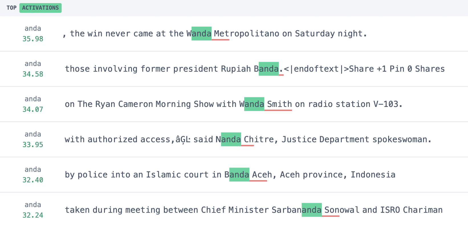
Consider feature 3.15566 examined in our previous post [AF · GW] covering all attention heads in GPT-2 Small, which activates on female pronouns and attends back to the name. We examine this feature on the prompt “Amanda Heyman, professional photographer. She”. On the final token, the source position DFA (step 2 in RDFA) indicates the model is attending backwards to the second token of Amanda’s first name, “anda”. 
 

While this tells us that information from the “anda” source position is being used to activate this attention SAE feature, we can use residual stream DFA to zoom in on the specific features that are being moved. Attributing the relevant resid_pre SAE feature (step 3 in RDFA) shows only a handful that are relevant at this source position.

Let’s example the top four features:

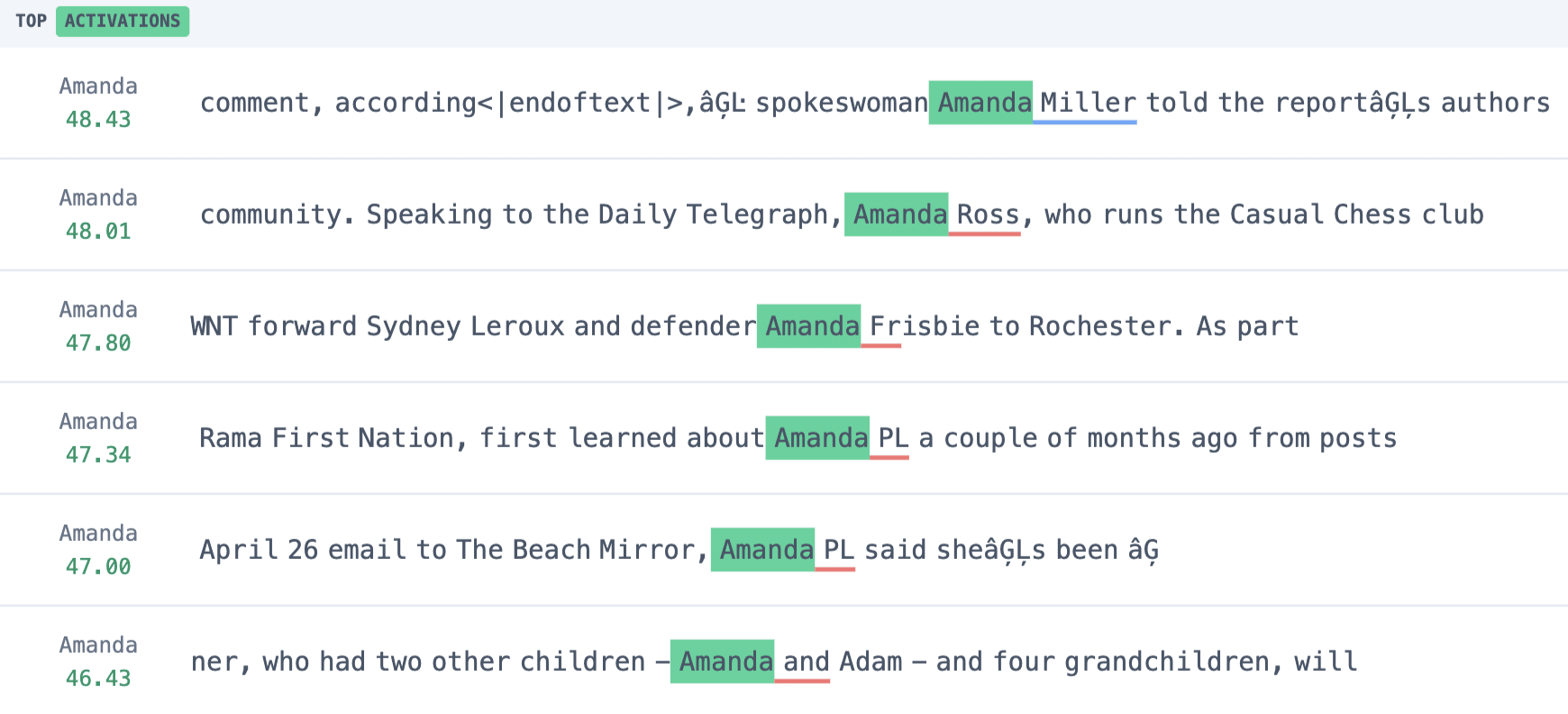
• Residual feature 3.19755: Activates maximally on names ending with “anda”. We note that these seem primarily female (e.g. Yolanda, Miranda, Fernanda, Wanda, etc.) 
  
• Residual feature 3.14571: Activates on the last token of multi-token female first names, and boosts last names more generally.
  
  

 

• Residual feature 3.14186: Specifically activates in “Amanda”, and boosts last names for “Amanda”
  

• Residual feature 3.1683: Boosts common last names on certain common names.

While we would need to deep dive into these features to confirm their interpretation, these are all reasonable signals to build as early as the second token based on the name “Amanda”. The fact that at the “she” token the model is mainly attending back to the second token on “Amanda” where it has these four features available is illustrative of how granular we can be with this technique to capture both how components retrieve information and what specific information is accessed.

Example: Retrieving "Dave" using recursive attention attribution.

Live Demo with Attention Circuit Explorer

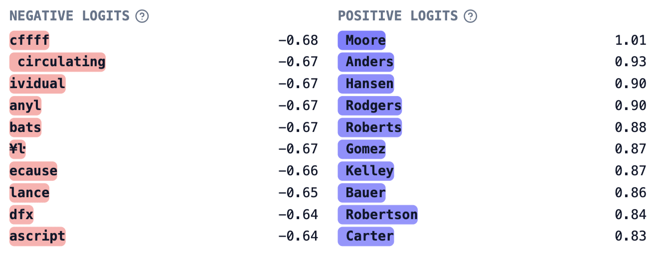
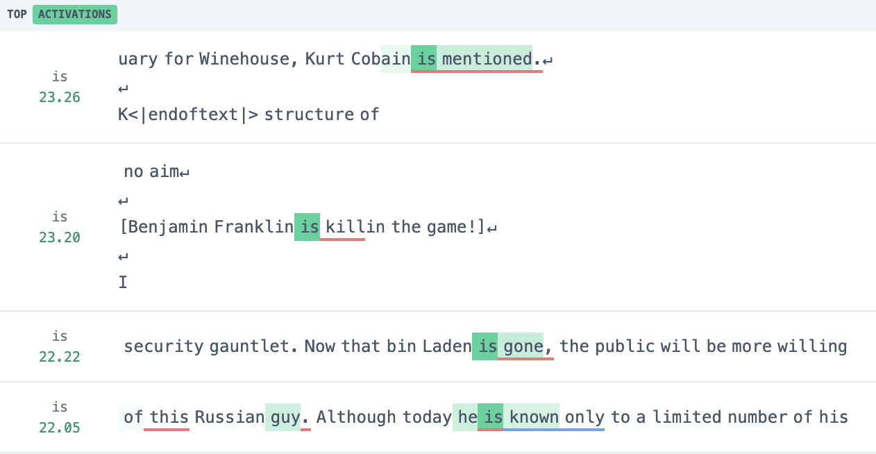
Consider the following example from the original ACDC paper: "So Dave is a really great friend, isn’t" (which was found by Chris Mathwin et al), where GPT-2 small is able to correctly predict the correct gender pronoun. We identify active attention output features such as 10.14709 which predicts tokens like "his" and "he". 

We now investigate this example using the RDFA tool to understand how this feature is computed. We start with DFA by source position to see what information is being moved to compute this feature. 

As expected based on the paper, the source position DFA indicates the model is attending backwards to the "is" token. Let's examine how this decomposes into resid_pre features:

Although the error term dominates, the other top resid_pre features are variants of usages of "is":

• Residual feature 10.1719: "specific mentions or actions related to individuals or their identities" particularly activating on "is" or "was".
• Residual feature 10.4075: "specific mentions or actions related to individuals or their identities" again particularly activating on "is" or "was.
  

Let's step into the second highest resid_pre feature 10.8758, which activates on tokens following names, to identify its attribution into upstream components: 

Although the majority of attribution is the Layer 5 MLP, we also see some attribution to Layer 2 and Layer 3 attention. Examining the top feature in Layer 2, A2.13775: 

It's a "Dave" feature! In fact, it is an "I follow Dave" feature which is even more interesting. We can see from this chain of observations using the tool that the model is routing information about "Dave" via the "is" token to the final "[isn]'t" position. 

Even Cooler Examples: Win a $1000 Bounty!

We are soliciting examples from readers and the public that demonstrate interesting attention-to-attention connections in GPT-2 Small. Open up the Circuit Explorer tool and let us know what you find. If there is an example you wish to submit, or if you run into any trouble or just want some help on how to use the tool, you can reach out to @robertzk [AF · GW] and @Connor Kissane [AF · GW] over an AF or LW direct message. The best example produced by 07/15/24 as subjectively assessed by the authors of this post will receive a $1,000 bounty.

Try the Attention Circuit Explorer and send us your feedback.

Related Work

This is a short research output, and we will fully review related work when this research work is turned into a paper. In the meantime, we recommend the Toy Models of Superposition related work section that covers background and proposed solutions in Dictionary Learning (the problem that SAEs solve), the Gated SAEs related work for a currently-up-to-date summary of SAE research, the Attention Superposition Anthropic update, which links to some Attention Head superposition work, which also attempts to interpret Attention Heads. He et al. also exploit the transformer’s linear structure to investigate composition between SAE features in Othello, similar to our RDFA approach. We were also inspired by Sparse Feature Circuits as this also uses SAEs for circuit analysis. 

In concurrent work, Ge et al., 2024 also find “ and”-related feature in the IOI task, and rediscover the induction feature family (Kissane et al., 2024 [LW · GW]). We causally verify the hypotheses of how “ and” features behave in IOI and rule out alternative hypotheses.

Conclusion

Overall, we remain tentatively optimistic about dictionary learning after this research. We found that, at their best, SAEs allow us to zoom in on a confusing part of the IOI circuit (despite lots of prior effort without SAEs) and immediately figure out what’s going on. We’re also excited that they enable new techniques like recursive DFA that allow us to better trace how features connect in a more principled way. 

On the other hand, our evaluations revealed that some of our SAEs were not viable to analyze certain sections of the IOI circuit, which we’ll need to address before SAEs can be a “silver bullet” for arbitrary circuit analysis. We also felt a bit constrained by only focussing on attention outputs, and while we remain excited about Attention Output SAEs, we’ll need additional tools to deal with MLP nonlinearities and QK circuits if we are to tackle more ambitious interpretability questions.

Limitations

• IOI is a relatively simple task that is already well understood. In the future we’re excited about applying SAEs to gain insight into more complex, safety relevant behaviors.
• We only did relatively shallow investigations of the causally relevant features, so we may be missing subtleties. Rigorously interpreting SAE features (Bricken et al.) is expensive, and properly interpreting SAE features at scale remains an open problem.
• Our recursive DFA technique fails to go back through MLP nonlinearities. We believe this can be addressed with techniques which we describe in future work.

Future Work

We intend to continue dictionary learning research. Some work streams include:

• Dealing with MLPs in circuit analysis. Recall that our recursive DFA technique treated mlp_out activations as leaf nodes. We could apply an MLP SAE to these activations, but even then we can’t use DFA to go back through the non-linear activation function. One approach is to apply causal interventions (e.g. path patch the MLP inputs) to get around this, but this loses the nice linearity of DFA. We’re alternatively excited about ongoing work attempting to decompose the MLPs with Transcoders (Dunefsky et al. [AF · GW]).
• Training better SAEs. Our SAEs were pretty useless for the later layers. Do we just need to train bigger / better SAEs, or are there more fundamental limitations of dictionary learning? We’re tentatively optimistic due to rapid progress in science / scaling from labs like GDM [AF · GW] and Anthropic. We’re particularly excited to see that Rajamanoharan et al. scaled Attention Output SAEs to a 7B parameter model. We’re also excited about progress in open source tooling (SAELens) which should make it easier for the community to train and open source better SAEs (Bloom [AF · GW]).
• Applying SAEs to more complex tasks. IOI is not a particularly interesting task. Can we apply SAEs to better understand more complex behaviors, like hallucinations?

Some additional directions that we think are particularly accessible (e.g. for upskilling projects) include:

• Apply SAEs to zoom in on other previously studied circuits, using similar techniques to this post. See Hanna et al. and Conmy et al. for some examples of circuits. Where are the SAEs viable for analysis vs where do they break things? What new things can you learn? Hopefully this should now be easy with HookedSAETransformer! 
• More rigorously interpreting SAE features. Can you more deeply understand how L5.F44256 is computed upstream? See Bricken et al. and our first post [AF · GW] for inspiration.

Citing this work

Feel free to use the citation from the first post [LW · GW], or this citation specifically for this current post: 

@misc{attention_saes_4,
  author= {Connor Kissane and Robert Krzyzanowski and Arthur Conmy and Neel Nanda},
  url = {https://www.lesswrong.com/posts/EGvtgB7ctifzxZg6v/attention-output-saes-improve-circuit-analysis},
  year = {2024},
  howpublished = {Alignment Forum},
  title = {Attention Output SAEs Improve Circuit Analysis},
}

Author Contributions Statement

Connor and Rob were core contributors on this project. Connor performed the IOI case study. Connor also implemented and open sourced HookedSAETransformer based on a design from Arthur, with significant feedback from Neel and Nix Goldowsky-Dill. Rob designed and built the tool to discover attention feature circuits on arbitrary prompts with recursive DFA, and performed automated circuit scans for examples of attention-to-attention composition. Arthur and Neel gave guidance and feedback throughout the project. The original project idea was suggested by Neel.

Connor would like to thank Keith Wynroe, who independently made similar observations about IOI, for helpful discussion.

Rob would like to thank Joseph Bloom for building the residual stream SAEs [AF · GW] that enabled the RDFA tool to pass through residual stream features and Johnny Lin for adding Neuronpedia functionality to enable just-in-time interpretation of these features. 

1. ^{^}

   We suspect that they might be missing features corresponding to the Negative Name Mover (Copy Suppression) heads in the IOI circuit, although we don’t investigate this further.

2. ^{^}

   We repeat this experiment with five other alternatives to ‘ and’ and observe similar effects. See the appendix

3. ^{^}

   We don’t write the LayerNorms for readability. In practice we fold LN, and cache and apply the LN scale

4. ^{^}

    In practice we stack the SAE decomposition into a matrix of shape [d_sae+2, d_model]

5. ^{^}

   Note we filter out features that never activate on these prompts

6. ^{^}

   Note we exclude SAE bias terms in this analysis

0 comments

Comments sorted by top scores.