Inside the mind of a superhuman Go model: How does Leela Zero read ladders?

post by Haoxing Du (haoxing-du) · 2023-03-01T01:47:20.660Z · LW · GW · 8 comments

Contents

  Introduction
  Prior work
  Setup
    Model
    The ladder behavior
    Dataset
    Methods
  Results: General properties
    Preferred basis and “logit lens”
    Edges of the board are used to store global information
    Value information is stored in checkerboard patterns
  Results: Ladder breaker detection
    Equivariance/Symmetry
    The circuit is pretty big …
    … but has a small, early bottleneck
    Breaker indicator ≠ ladder detector
  Conclusion and future work
  Acknowledgement
  Citation information
  Appendix A: Details on policy head
  Appendix B: Details on value head
  Appendix C: Algorithmic tasks in Go
    Identifying legal moves
    Escaping atari
    Counting territories
None
8 comments

tl;dr—We did some interpretability on Leela Zero, a superhuman Go model. With a technique similar to the logit lens, we found that the residual structure of Leela Zero induces a preferred basis throughout network, giving rise to persistent, interpretable channels. By directly analyzing the weights of the policy and value heads, we found that the model stores information related to the probability of the pass move along the top edge of the board, and those related to the board value in checkerboard patterns. We also took a deep dive into a specific Go technique, the ladder, and identified a very small subset of model components that are causally responsible for the model’s judgement of ladders.

Introduction

We live in a strange world where machine learning systems can generate photo-realistic images, write poetry and computer programs, play and win games, and predict protein structures. As machine learning systems become more capable and relevant to many aspects of our lives, it is increasingly important that we understand how the models produce the outputs that they do; we don’t want important decisions to be made by opaque black boxes. Interpretability is an emerging area of research that aims to offer explanations for the behavior of machine learning systems.

Early interpretability work began in the domain of computer vision, and there has been a focus on interpreting transformer-based large language models in more recent years. Applying interpretability techniques to the domain of game-playing agents and reinforcement learning is still relatively [LW · GW] uncharted territory. In this work, we look into the inner workings of Leela Zero, an open-source Go-playing neural network. It is also the first application of many mechanistic interpretability techniques to reinforcement learning.

Why interpret a Go model? Go models are very capable. Many of us remember the emotional experience of watching AlphaGo’s 2016 victory over the human world champion, Lee Sedol. Not only have there been algorithmic improvements since AlphaGo, these models improve via self-play, and can essentially continue getting better the longer they are trained. The best open-source Go model, KataGo, is trained distributedly, and the training is still ongoing as of February 2023. Just as AlphaGo was clearly one notch above Lee Sedol, every generation of Go models has been a decisive improvement over the previous generation. KataGo in 2022 was estimated to be at the level of a top-100 European player with only the policy, and can easily beat all human players with a small amount of search.^[1] Understanding a machine learning system that performs at a superhuman level seems particularly worthwhile as future machine learning systems are only going to become more capable.

Little is known about models trained to approximate the outcome of a search process. Much interpretability effort have focused on models trained on large amounts of human-generated data, such as labeled images for image models, and Internet text for language models. In constrast, while training AlphaZero-style models, moves are selected via Monte-Carlo Tree Search (MCTS), and the policy network of the model is trained to predict the outcome of this search process (see Model [LW(p) · GW(p)] section for more detail). In other words, the policy network learns to distill the result of search.^[2] While it is relatively easy to get a grasp of what GPT-2 is trained to do by reading some OpenWebText, it’s much less clear what an AlphaZero-style model learns. How does a neural network approximate a search process? Does it have to perform internal search? It seems very useful to try to get an answer to these questions.

Compared to a game like chess, mastering the game of Go is more likely to require spatial generalization and crisp algorithms. In chess, having a pawn on d4 is an entirely different position than a pawn on e4, and the fact that simple techniques such as piece-square tables work reasonably well suggests that perhaps much of the game can be learned by memorizing specific positions, and does not require generalizing to broad heuristics. Go, on the other hand, with its bigger board size and only one type of piece, is intuitively much more conducive for the model to learn general algorithms. For example, the model had better have the concept of the number of liberties that a group has, no matter where the group is on the board and the group’s size and shape. As we explain more below, algorithmic behaviors are in our view great candidates to study with interpretability, and this is a main reason we focus on the game of Go.

Another motivation for interpreting these models is that they are not very big. Having had some success with interpreting large language models, the most capable Leela Zero network at 47 million parameters, or just over 1/3 of the parameter count of GPT-2 small (117 million), the smallest of the GPT-2 family, seems pretty well within reach. Last but not least, interpreting Go models started making sense because we have developed a set of tools from studying language model interpretability that we believe are universally useful, and we felt that it was time to apply them to other domains. For example, path patching allows us to precisely isolate the effect of every causal pathway in the model, and causal scrubbing [? · GW] enables us to evaluate interpretability claims in a rigorous and principled way. This work is a proof of concept for these techniques and ideas, and in turn we felt that we were ready to tackle interpretability questions in a new domain with these tools under our belt.

We found a number of general properties of Leela Zero:

• The residual structure, even with a ReLU nonlinearity in between every layer, is strong enough to induce a preferred basis throughout the model. This means that information about a particular position on the board stays at that position, and information in a particular channel stays in that channel and gets refined layer by layer.
• We are able to get a good understanding of how the policy and value heads [LW(p) · GW(p)] work by directly examining the weights, and found that the model stores global information about the game state with regular patterns. In particular, we found that the top edge of the board is used to store information about the pass move, and used this knowledge to manipulate the model into assigning twice the probability to passing than it otherwise would.
• We found that the information about the value of the board (i.e. which player is predicted to win) is stored in checkerboard-like patterns. To our knowledge, this is the first time checkerboard patterns are observed in convolutional neural networks with no strided convolution or pooling.

Lastly, we focus on a particular algorithmic behavior in Go—detecting ladder breakers—and identify a small subset of the model are causally responsible for this behavior. We found a single channel that is overwhelmingly important for the behavior that appears very early in the model, essentially as early as it is possible to appear as constrained by the receptive fields of neurons. This is a first step towards the mechanistic understanding of a sophiscated behavior of a real-world machine learning system.

Prior work

There has been a relatively well-established line of research on explainability in reinforcement learning and some effort to apply interpretability techniques to RL, but the work most closely related with this project was published in 2022 by DeepMind and Google Brain, titled “Acquisition of Chess Knowledge in AlphaZero”. The focus of the paper is on the representation of human chess concepts. With techniques such as linear probes, the authors demonstrate that AlphaZero employs many human chess concepts, and show where they are represented in the network, as well as when they are formed in training. Although similar in theme, this project takes quite a different angle. Instead of concept-based interpretability, we aim to provide a mechanistic explanation for how Leela Zero implements a specific algorithm. In this sense, this work is more closely related to some previous work in language model interpretability.

A direct influence on this project has been Wang et al’s work on Indirect Object Identification (IOI) in GPT-2. The authors investigated an algorithmic task in natural language—the task of inferring the indirect object of a sentence—and identified a circuit responsible for the behavior. Inspired by this work, we chose to focus on an algorithmic task in Go. We also relied heavily on the techniques developed from the IOI work, in particular activation patching, and a specialized version of it called path patching. We elaborate on both of these points in the Methods [LW(p) · GW(p)] section below.

Our work is also inspired by the image model interpretability work pioneered by Chris Olah, especially Circuits-style mechanistic interpretability. However, while Circuits-style work aims to reverse-engineer the behavior of neural networks in generality, here we focus on explaining the model’s behavior on a specific distribution. This is both due to practical concerns (as Leela Zero has ~10x the parameter count of InceptionV1, a general, mechanistic understanding of it is almost certainly intractable with current techniques), and also because we believe that understanding the model’s behavior on a narrow distribution teaches us valuable lessons. Another difference is that in this work, we focus on establishing the causal relationship of model components, and validate our claims with causal scrubbing. This allows us to make interpretability claims that go beyond human-understandable concepts and quantitatively assess the validity of these explanations.

Setup

Model

For this project, we were interested in AlphaZero-style models for the game of Go.^[3] These are models that use Monte-Carlo Tree Search guided by a policy network (i.e. a network that predicts the goodness of possible moves) and a value network (i.e. a network that predicts the goodness of the board position), and trained entirely via self-play. None of the DeepMind models is publicly available, but the computer Go community has worked hard to produce open-source models trained with the AlphaZero algorithm. The two best open-source Go models currently are KataGo and Leela Zero. Leela Zero is essentially an exact replication of the AlphaGo Zero paper, while KataGo pioneered a number of changes on top of the AlphaZero algorithm to make it especially adapted to playing Go. KataGo is still an ongoing project, while the Leela Zero project was halted in 2021. At this point, KataGo is more popular and likely quite a bit stronger.

However, we focused on Leela Zero instead of KataGo, and this is also because of the handcrafted, Go-specific features that KataGo uses. While features such as the number of liberties at each intersection and ko restrictions help KataGo learn to play Go a lot faster and better, they make a lot of the interpretability problems [LW · GW] we were interested in less interesting—the “moving here catches opponent in ladder” feature certainly makes the ladder behavior uninteresting. So we opted for using Leela Zero in our investigation so far; that said, we think that it would be interesting study KataGo with interpretability tools as well, and it would be very interesting to see whether the two models have internal mechanisms that are at all similar.

Leela Zero is an exact replication of AlphaGo Zero, with just one modification, as we explain below. It is essentially a ResNet with a policy head and a value head, and takes only images of the board state as input. The most capable model has 40 residual blocks with 256 channels. It takes as input 18 19x19 binary feature planes, with 19x19 being the standard size of a Go board. The first eight 19x19 features indicate the positions of the current player’s stones from the last eight time steps, and the next eight indicate the positions of the opponent’s stones from the last eight time steps. The second to last 19x19 array is all ones if black is to move, and all zeros otherwise; the last feature is all ones if white is to move, and all zeros otherwise. The original AlphaGo Zero only had 17 feature planes, with only one plane indicating which side is to move. It turns out that although conceptually equivalent, this causes a slight bias favoring black, because the convolutional layers use zero-padding.^[4] So Leela Zero added an additional feature plane to fix the asymmetry between black and white, and this is the only way it differs from AlphaGo Zero. The output of the policy head is a single 19 * 19 + 1 = 362 dimensional array, where the first 361 entries are logits for each move on the board, and the last entry is the logit of passing. Probabilities are obtained after normalizing with softmax. The value head outputs a single number, with +1 meaning the current player is expected to win, and -1 meaning the opponent is expected to win.

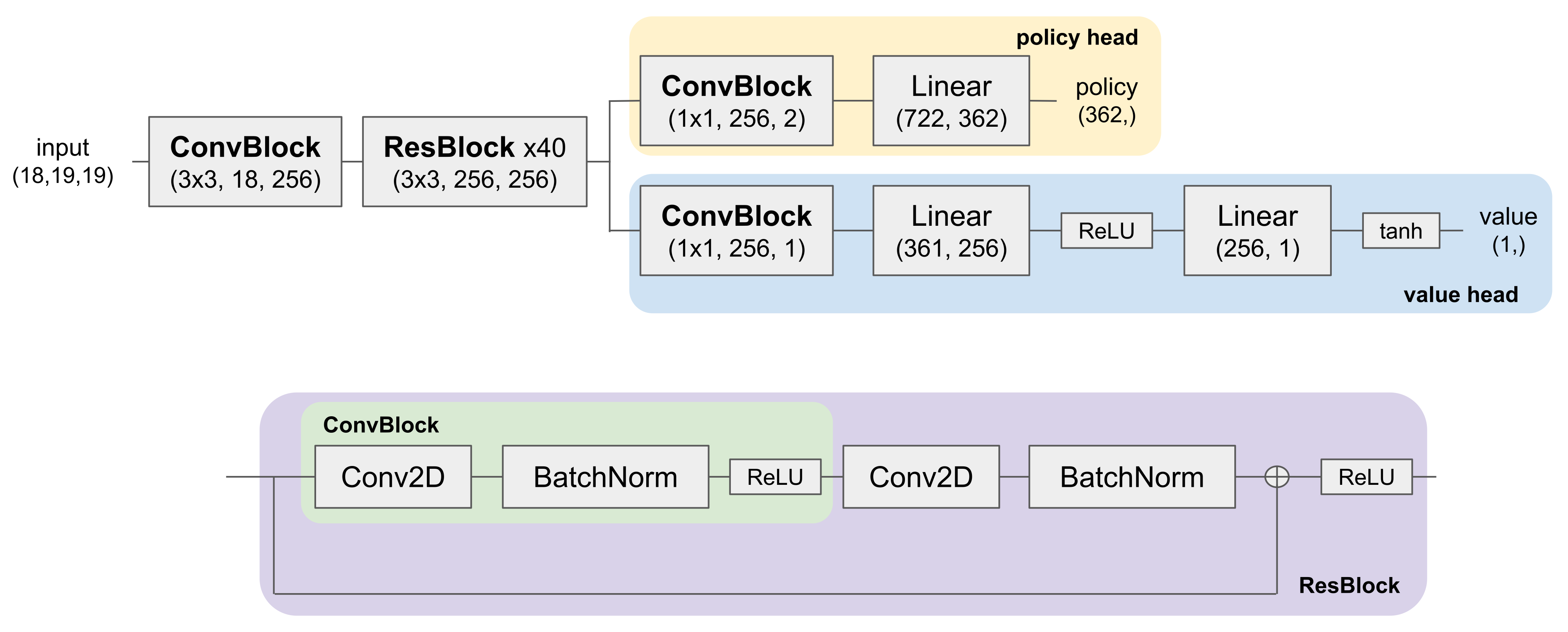
When in training—and deployed in real games, as the training process just involves playing copies of the model against each other—moves are selected via MCTS using both the policy and value heads. The policy head is trained to predict the output of MCTS, and the value head is trained to predict the outcome of the game at every board position. In training, Leela Zero used up to 1600 search steps per move; in deployment, there is no limit to how many steps of search to use, and it is not uncommon to use millions of steps in a real game. For this project, we did not interact with MCTS at all, and just focused on the internals of the neural network.

The ladder behavior

In language model interpretability, one way of making progress had been to “pick the low-hanging fruit”: The full form of language is incredibly complex. The language we speak and write is a balance between many different considerations, a mix of many different heuristics, and context-specific judgements. To achieve a low loss on next-token prediction, it’s very likely that a good language model is also doing all of these things in its internal computations. If we want to make progress on interpretability, it seems much easier to focus on narrow distributions that enlarge one specific heuristic that the language model uses. These are sometimes referred to as algorithmic tasks. The Indirect Object Identification (IOI) task is such an example: When prompted “Yesterday, John and Mary went to the store, Mary gave an apple to”, the model completes “John” much more often than “Mary”. Wang et al are able to discover the underlying circuit for this specific behavior.

We face the same problem in Go. If you have played a few games of Go, you would realize that much of the beauty of the game lies in global strategic thinking, and playing a good game of Go requires constant balancing and prioritizing of the different regions of the board. A superhuman Go model is likely doing the same internally, and it’s natural to look for algorithmic tasks in Go as a starting point of digging into the model’s internals.

What is an algorithmic task in Go? In Appendix C [LW · GW] we provide several more examples, but here we will focus on one particular task: detecting ladder breakers.^[5]

The ladder is a common pattern in Go, and the name comes from the staircase-like shape formed by the stones on the board. The ladder is a great technique for the attacker, because once it’s initiated, every move the attacker plays forces the defender to respond and continue the ladder, until it hits the edge of the board, at which point the attacker captures all of the stones surrounded by the ladder.

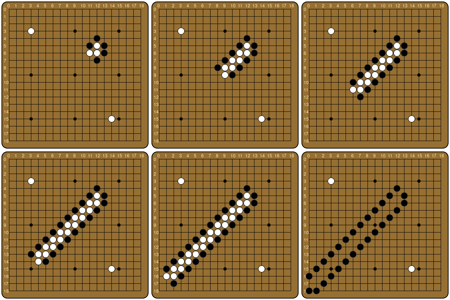
This is broadly true, unless there is a ladder breaker. Ladder breakers can come in arbitrarily complex forms, but the simplest is a single of the defender’s stones somewhere along the future trajectory of the ladder. When that is the case, the defender can escape once the ladder hits the breaker, essentially gaining an extra turn. Therefore, ladders are great for the attacker to play out, unless there is a ladder breaker.

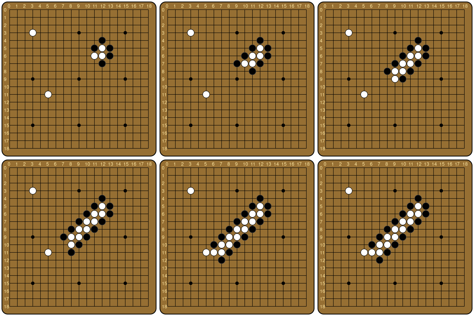
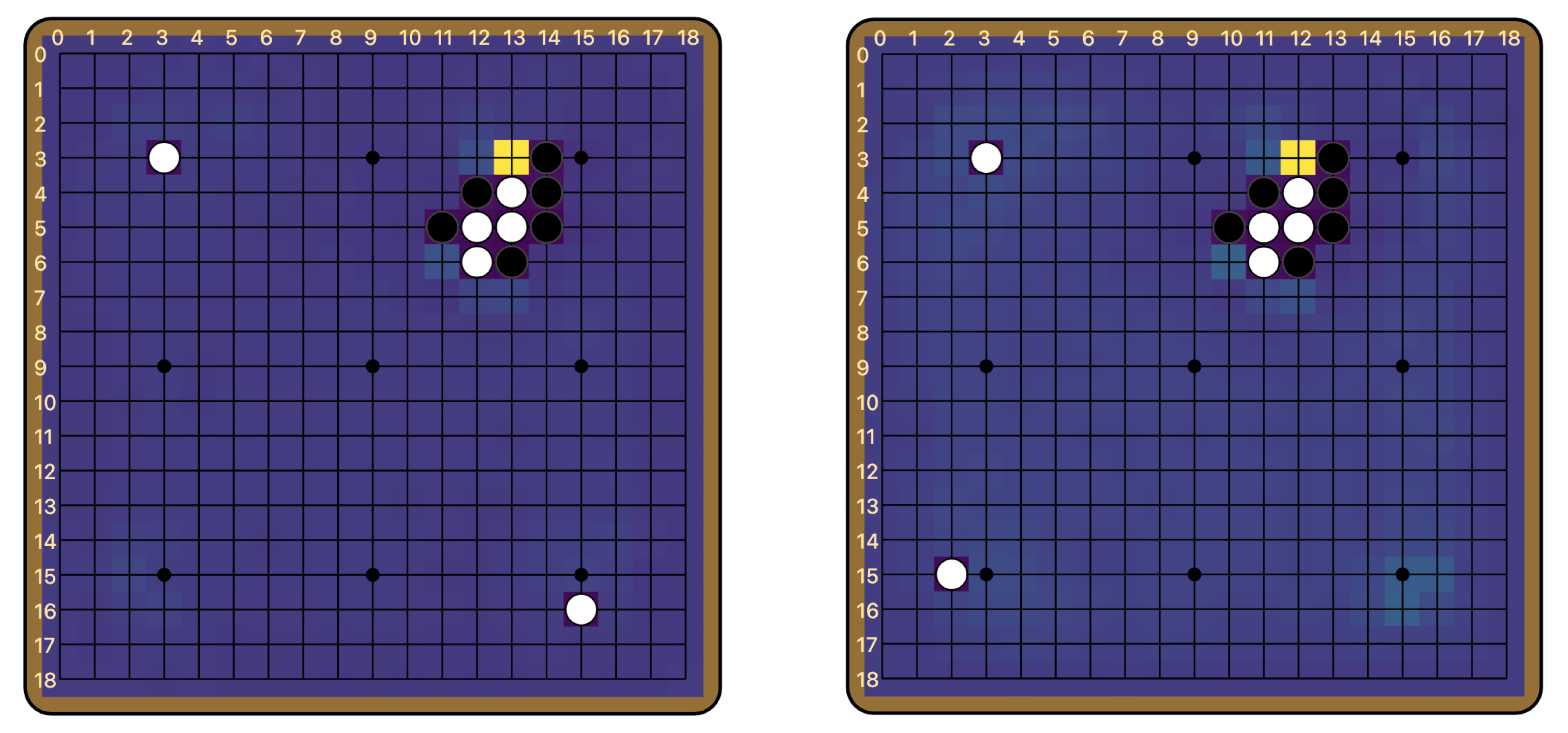
The ladder is not a difficult concept to grasp for most human beginners, but it is famously difficult for Go-playing AIs. From the original AlphaGo to KataGo today, many Go models rely on an external program to compute the outcome of ladders. Leela Zero does not have any explicit features about ladders, but can nevertheless judge ladders, at least the simple ones. Below is the output of Leela Zero’s policy network, for boards with and without a ladder breaker. We see that Leela Zero judges the move of continuing the ladder to be better when there is no breaker.

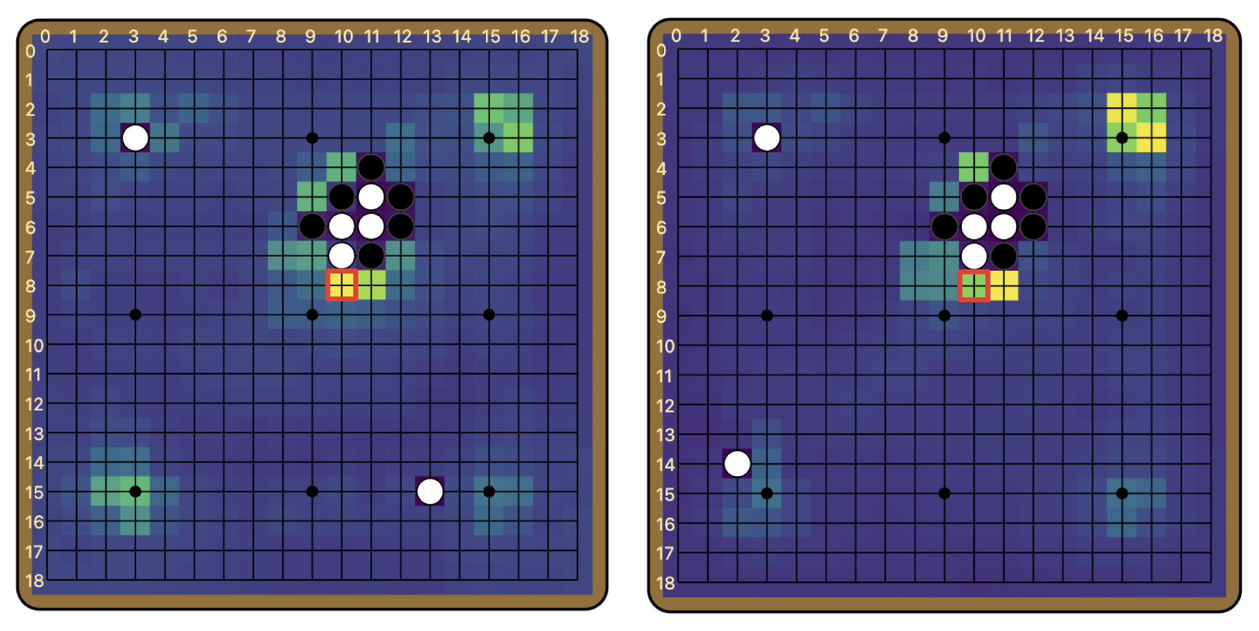
This behavior hints strongly at an underlying algorithm, and suggests a number of interesting questions to attempt to answer with interpretability.

Dataset

We made a dataset that consists of ladder positions with and without breakers. Specifically, whenever we generate the start of a ladder, we add one board with breaker and one board without breaker to our dataset. The starting position of the ladder, the position of the breaker, and ladder starting length can all vary.^[6] We fix that black is the attacker (i.e. is on the outside) and fix the board to be in a state where black is to move. Note that the model does not have black or white stones as a concept, and instead only thinks of the stones as “own’s stones” and “opponent’s stones”, so we can do this without loss of generality. We measure the log probability assigned by the policy head to the move that continues the ladder. For example, the figure above is a pair of boards from our dataset, one with a ladder breaker and one without.

Averaging over a dataset of 50 pairs of such boards, we get that the mean log probability assigned to the ladder move when there is no ladder breaker is -0.925 (probability 39.7%), and that when there is a breaker is -3.375 (probability 3.4%).

Methods

Other than direct examination of the weights and visualization of activations, a main technique we use in this work is activation patching, which means replacing a part of the model’s forward pass with activations from a different input. First invented by Vig et al for causal mediation analysis in language models, we favor it precisely because it reveals the causal relationship between parts of the model.

We use the following metric to report the result of patching experiments: We measure the default log probability of the ladder move both with and without a breaker, and call it log_prob_b and log_prob_nb. In patching experiments, we patch some breaker activations into the forward pass for the board with no breaker. If the location that we patch at is not important for this behavior, then we would see a resulting log probability that is essentially the same as log_prob_nb. If the location(s) patched were responsible for the entirety of the difference between the breaker and no breaker cases, then we would see a resulting log probability that is essentially the same as log_prob_b. Thus, we report the effect of any particular patching experiment as a percentage, (patched_log_prob - log_prob_nb)/(log_prob_b - log_prob_nb), with 0 meaning the patch had no effect, and 100% meaning that the patch is responsible for the whole effect.

This methodology is closely linked to causal scrubbing, a method [? · GW] for quantitatively testing the validity of interpretability claims. Say that we identified a set of model components that are responsible for the ladder behavior—how would we know how good our answer is? One intuitive metric is: If our answer is good, that is, if we have identified all of and only the components of the model that matter for this behavior, then running the model on only this subset of components should be as good as running the whole model. To test this, we turn the rest of the model “off”. There are many methods for doing this in the literature, such as zero ablation and mean ablation. We take the in our view more principled approach of resampling ablation—running unimportant parts of the model on a different input. Thus, in causal scrubbing language, patching a part of the model is the same as resampling-ablating the rest of the model, and our metric is a special case of the “percentage of loss recovered” [LW · GW] metric used in most causal scrubbing results.

We also perform an algebraic rewrite on the model which we call residualification. As we show below [LW · GW], Leela Zero behaves very similarly to a residual network, and it only differs from a true residual network by a ReLU in between every block. Consider the following rewrite: Define $\tilde{f}\left(x\right)$ such that $x+\tilde{f}\left(x\right)=\text{ReLU}(x+f(x\left)\right)$. Then

$$\tilde{f}\left(x\right)=\{\begin{array}{cc}f\left(x\right)& \text{if}x+f\left(x\right)>0,\\ -x& \text{otherwise.}\end{array}$$

Then our model is a true residual network in terms of the $\tilde{f}$’s. And if it is the case that the ReLU functions as the identity most of the time, then $\tilde{f} = f$ in the majority of the cases.

Once we have rewritten the model this way, we can now conduct path analysis on this model. When there are skip-connections in the network, the network can be “unraveled” and the output can be written as a sum over contributions from different paths. This type of analysis has been extensively used in both vision and language models. Path patching is a technique developed from the IOI work, which allows us to isolate the effect of any particular path. For example, in a three-layer residual network as shown in the diagram below, there are eight distinct paths of information flow from the input to the output. Regular activation patching affects all paths that involve a certain component. For example, patching layer 0 affects all of the yellow paths. In contrast, path patching singles out the effect of a particular path, allowing us to isolate the effect of e.g. the blue path, which is the direct path from layer 0 to layer 2.

Results: General properties

Preferred basis and “logit lens”

In GPT-2, it has been shown that the activations at intermediate points in the model resemble those at the last layer, and multiplying them by the unembed matrix gives logit distributions not far off from the actual output. This is the technique termed the logit lens [LW · GW]. This is believed to be due to the residual structure of transformers: the output of each layer is added to a residual stream, which is read in by later layers. The fact that the logit lens works is evidence towards the conceptual picture of transformers “iteratively refining a guess” for the next token.

Leela Zero, which shares most of its architecture with a ResNet, is also a residual network. The main difference with a transformer is that there is a rectified linear unit (ReLU) nonlinearity after the residual connection, as shown in the diagram above [LW(p) · GW(p)]. That is, if a layer implements the function $f$, the output after the layer is $\text{ReLU}(x+f(x\left)\right)$ instead of $x+f\left(x\right)$ as in transformers.

But apart from this one difference, Leela Zero’s architecture shares quite a lot of similarity with transformers, especially if one thinks of the first convolution block as a sort of embedding, and the policy/value head as a sort of unembedding. Can we also think of the layers of Leela Zero as iteratively refining a guess about the policy and value? A priori, it seems that the nonlinearity after each residual block might complicate things. But there is also a clear residual structure throughout the entire network, and the common wisdom is that ResNets are effective because each layer only needs to learn deviations from the identity function, and not identity itself.^[7]

A technique similar to the logit lens provides some answers. Instead of the unembed matrix, we take intermediate activations after each residual block (also referred to as layer; we will use the two terms interchangeably), and put it through the policy head. The question we are interested in is: How similar are the outputs from this process to the actual policy output? We can simply plot the result we get from each layer.

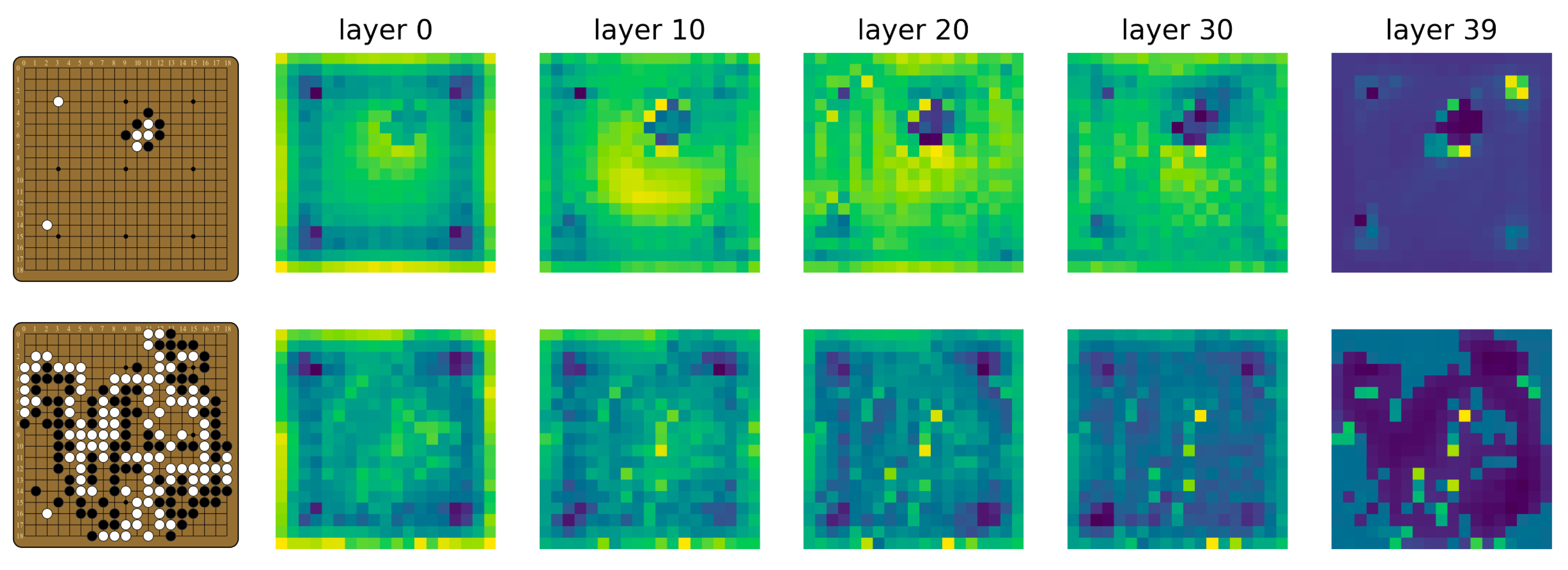
A few things to note here: First of all, the shape of the board is recognizable, even at layer 0. Despite being overall quite different from the final policy, earlier outputs seem to at least encode information about the board state. Second, the moves that end up with the highest logits in the final policy start to stand out fairly early on. For both boards, the brightest pixels in the layer 10 output are already pretty much the most likely moves in the final policy. Finally, there is a fair amount of noise in the output, and the output does not become that similar to the final policy until after layer 30. To characterize the overall trend of similarity, we calculate the Kullback-Leibler (KL) divergence between the logit lens output at each layer and the final policy. The plot below is averaged over 50 random boards from real games, with error bars.

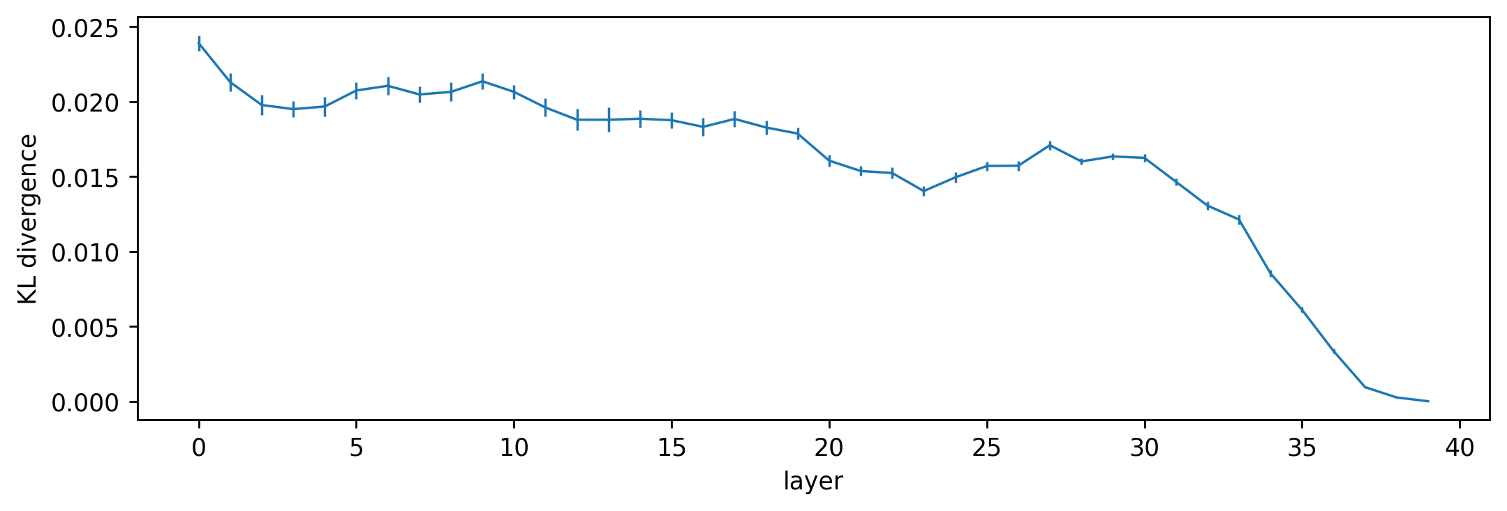
It seems that the logit lens works reasonably well on Leela Zero. The fact that the policy head applied to intermediate activations gives recognizably policy-like output means that the residual structure of the network induces a sort of preferred basis throughout the network, along both the board-position dimension and the channel dimension. In other words, information about the board position (i, j) seems to stay in the (i, j) entry,^[8] and information held in a particular channel for the most part stays in that channel,^[9] throughout the model. Furthermore, intermediate activations look much more like the output than the input. This affirms the picture that the layers of Leela Zero are reading from and writing to a “residual stream”.

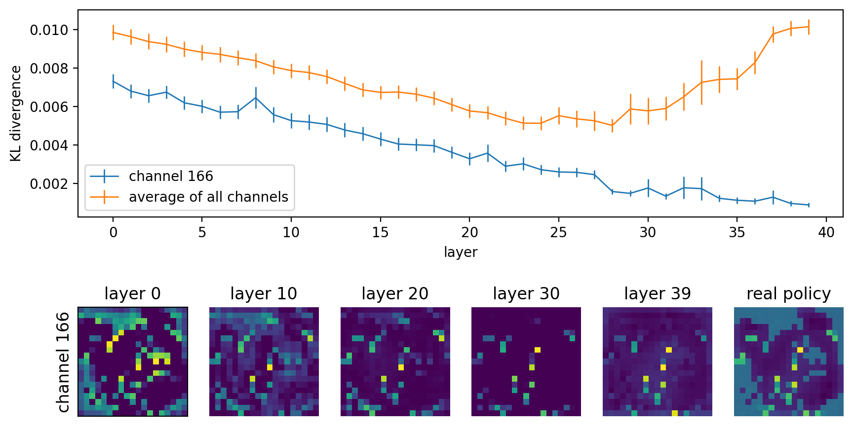
We are able to identify many channels which hold human-understandable information. For example, there are channels that simply retain the positions of each player’s stones throughout the whole model. One nice aspect of Leela Zero is that the architecture of the policy and value heads is very simple, and we can directly examine the weights and figure out how the policy is calculated from the features produced by the residual tower, i.e. the 40 ResBlocks. From this, we identified one channel, channel 166, as directly providing information about the best moves. See Appendix A [LW · GW] for more details on how we found channel 166.

The figure below shows the activations in channel 166 at various layers for the second board shown above. We see that even at layer 0, the activations have a clear correspondance with the policy—only unoccupied intersections on the board are active. We again use the KL divergence to quantify the degree of similarity with the policy. Since the claim is that activations in channel 166 are analogous to logits, and logits are not invariant under scaling, we learn a multiplacative scaling factor at each layer that minimizes the KL divergence of the channel activations from the policy across 50 boards. To show that the low KL divergence is not due to picking special scaling factors, we do this for both channel 166 and the average activations across all channels. This is further evidence for channel persistence as discussed above.

Edges of the board are used to store global information

Much of the model’s goal is to predict the optimal policy, that is, an optimal probability distribution over all the moves. In Go, the legal moves at any given point are all the empty intersections on the board (modulo ko restrictions and suicide moves), and passing. As discussed above, the model has the natural choice of storing information about the (i, j) intersection with the (i, j) entry in the activation. But how does the model represent the goodness of the pass move, which is a global property of the entire board?

Also by examining the weights of the policy head, we found that the model uses the top edge of the board to store information about passing. As a result, some features are actually shifted down by one row compared to the actual positions on the board—that is, information about intersection (i, j) is stored in the (i, j+1) entry of the activation—so that stones placed on the first line do not interfere with the information about the pass move.^[10] For example, the image on the left is channel 24 in layer 39, and the image on the right is channel 166 in layer 39. We know that channel 166 resembles the policy output, and we see that channel 24 resembles 166 except that all the positions are shifted downward by one row.

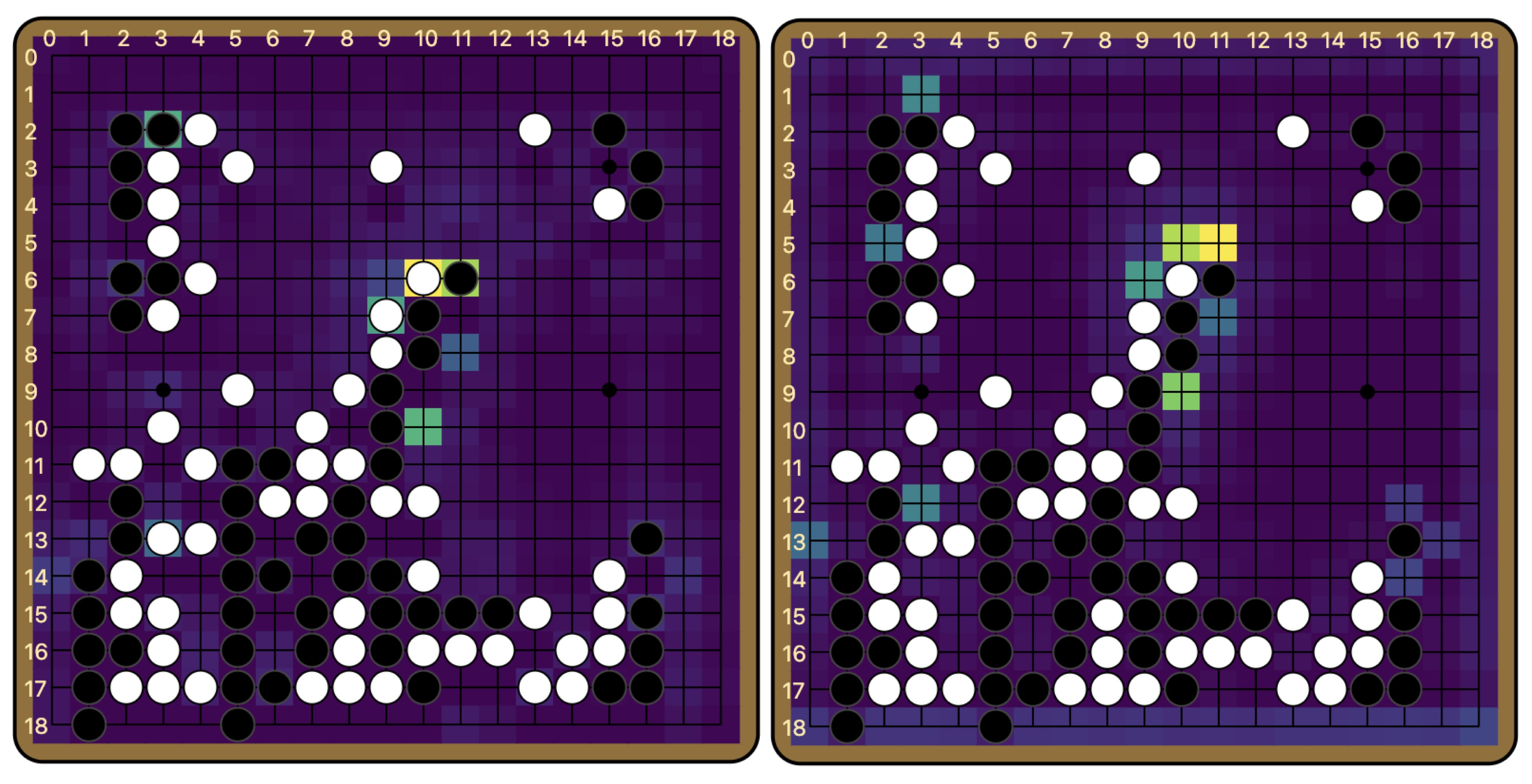
As we explain in Appendix A, [LW · GW] it turns out that the pass logit is mostly computed from information in the first row of the shifted features, but features that are not shifted also weakly contribute, and in an uneven way. In particular, the third row from the bottom contributes much more than other places on the board. This implies a testable claim: boards that have higher activations in the third to last row should cause the model to assign a higher probability on passing. It is not very clear what kinds of boards result in high activations at a particular position, but we know that at least some features resemble the policy, and we can make up artificial board positions that put a lot of probability on moves in the third to last row.

Consider the four board positions below. Go is a game with complete rotational and reflectional symmetry, and these four board positions should be equivalent. Indeed, the policy output looks essentially the same across the four boards. However, since we know that the model’s internal representation breaks rotational symmetry, we predict that the first of these boards causes a higher pass probability than the rest. Indeed, the first board results in a pass probability that is about 2-3 times that of the other boards. Although fairly artificial, this is a clear victory of interpretability: understanding the model’s internals enabled us to make concrete predictions about the model’s behavior that would be otherwise hard to discover.

In hindsight, storing global information about the game state along the edges of the board makes sense, as the edges are less frequently used than other parts of the board in most games of Go. But this is by no means an obvious choice a priori. In fact, the four corners of the board are used even less frequently. Why did the model not learn to use the corners instead, which would be more efficient and interfere with the board state even less? The model appears to use the other edges of the board as well, as it is fairly common to observe activations that highlight the other edges of the board. We think some of these are related to the value prediction (see below), but we don’t have concrete hypotheses for what they represent. There is of course the questions of how: How does the model compute the goodness of passing, and how does that information end up at the top edge? We leave these as future research directions.

Value information is stored in checkerboard patterns

Another piece of global information the model needs to keep track of is the board value. Recall that the value head computes the board value using the same set of features outputted by the residual tower as the policy head. The value head is only slightly more complicated than the policy head, and by examining the weights of the value head layers directly, we also learn how information about the board value is represented inside the model.

As detailed in Appendix B [LW · GW], separate features contribute positively and negatively to the evaluation. In particular, positive and negative value information are stored at different positions on the board, both in checkerboard-like patterns. Note that the two checkerboards are offset from each other by one column. This explains the checkerboard-like activations we frequently observed.

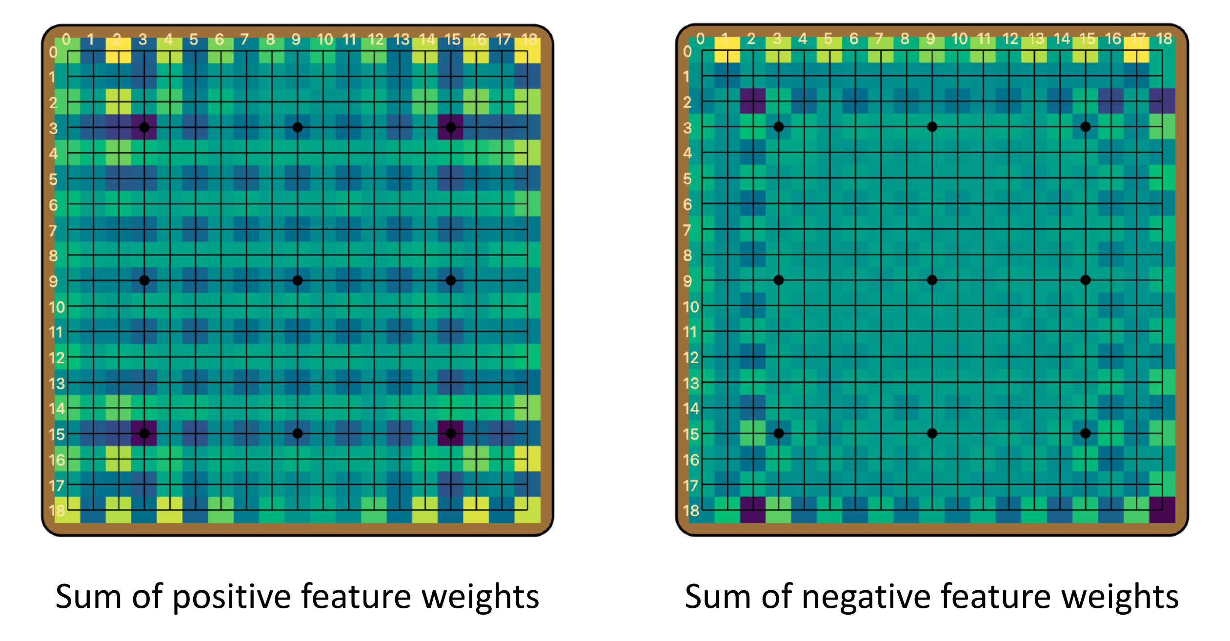
Famously, convolutional neural networks (CNNs) are prone to checkerboard artifacts, especially when used in image generation. Checkerboard-like noise was known to cause problems for feature visualization, and projects such as DeepDream had to employ techniques to dampen these artifacts. In 2016, Odena et al analyzed the causes of such checkerboard patterns, and attributed them to strided convolutions (it is technically deconvolutions, but even when there are no deconvolutions in the forward pass, gradients are essentially computed with deconvolutions in a backward pass). Certain less regular, high-frequency artifacts were also previously linked to max-pooling layers. But Leela Zero has no strided convolutions or pooling layers anywhere. As far as we are aware, the checkerboard patterns in Leela Zero are a novel phenomenon that is yet to be explained, and it shows that perhaps we still don’t fully understand checkerboard artifacts in CNNs. It is also very interesting to see that in this case, the model learns to take advantage of these “artifacts”, and use them to store global information.

Results: Ladder breaker detection

REMIX residents Naomi Bashkansky and Oliver Hayman contributed to this part of the project.

Equivariance/Symmetry

First, a comment about equivariance. Leela Zero, just like all convolutional neural networks, is not equivariant by design. While it is obvious to a human that an upside-down dog is still a dog, there is nothing in the CNN architecture that encodes this knowledge, and helps it learn naturally occurring symmetries. It is well-known that image models learn separate feature detectors for dog heads of different orientations, and Leela Zero does the same with Go. While Go is a game with full rotational and reflectional symmetry, Leela Zero doesn’t “know” that, and has to learn the symmetry from training.

In the case of ladders, there are four possible directions for the ladder to play out.^[11] Indeed, the model achieves similar performance for all four orientations, but has separate mechanisms for dealing with them. Below we specialize in one direction, which we happened to investigate first: the upper-right to bottom-left direction.

The circuit is pretty big …

As discussed above, we want to know how the model reads ladders. In other word, we want to uncover how the model implements the following logic: if there is a ladder breaker, ladder is bad; otherwise ladder is good.

One immediate question is: How big is this circuit? That is, is most of the model involved in producing this behavior, or is it fairly concentrated? An initial experiment we conducted is to patch each of the 256 channels at every layer and observe its effect. We found that there are 13 channels that have less than 0.1% effect when patched, and 91 channels that have effect between 0.1% and 1% when patched. This suggests that a major part of the model is not at all involved in this behavior.

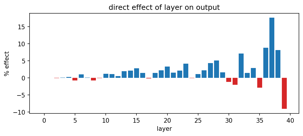
Experiments at the layer-level can help us clarify the conceptual picture. For example, we used path patching to measure the direct effect of each layer’s output on the metric. We see that early layers (before layer 10) essentially have no direct effect on the output, and the direct effect size increases towards later layers. There are a few layers (17 and 24) that appear to have no effect, but most middle layers contribute a little. This result also shows that residualification is a meaningful operation on this model. If we residualified a fully connected model, we would observe only the last layer having direct effect on the output. One other interesting thing is that some late layers in the model have the opposite effect on the behavior (i.e. make the model less confident about the ladder move when there is no breaker). Similar behavior is observed in the IOI work, and one interpretation is that the model is doing “calibration”, so as to not be overconfident with its output. It remains an open question how valid and how universal the calibration hypothesis is.

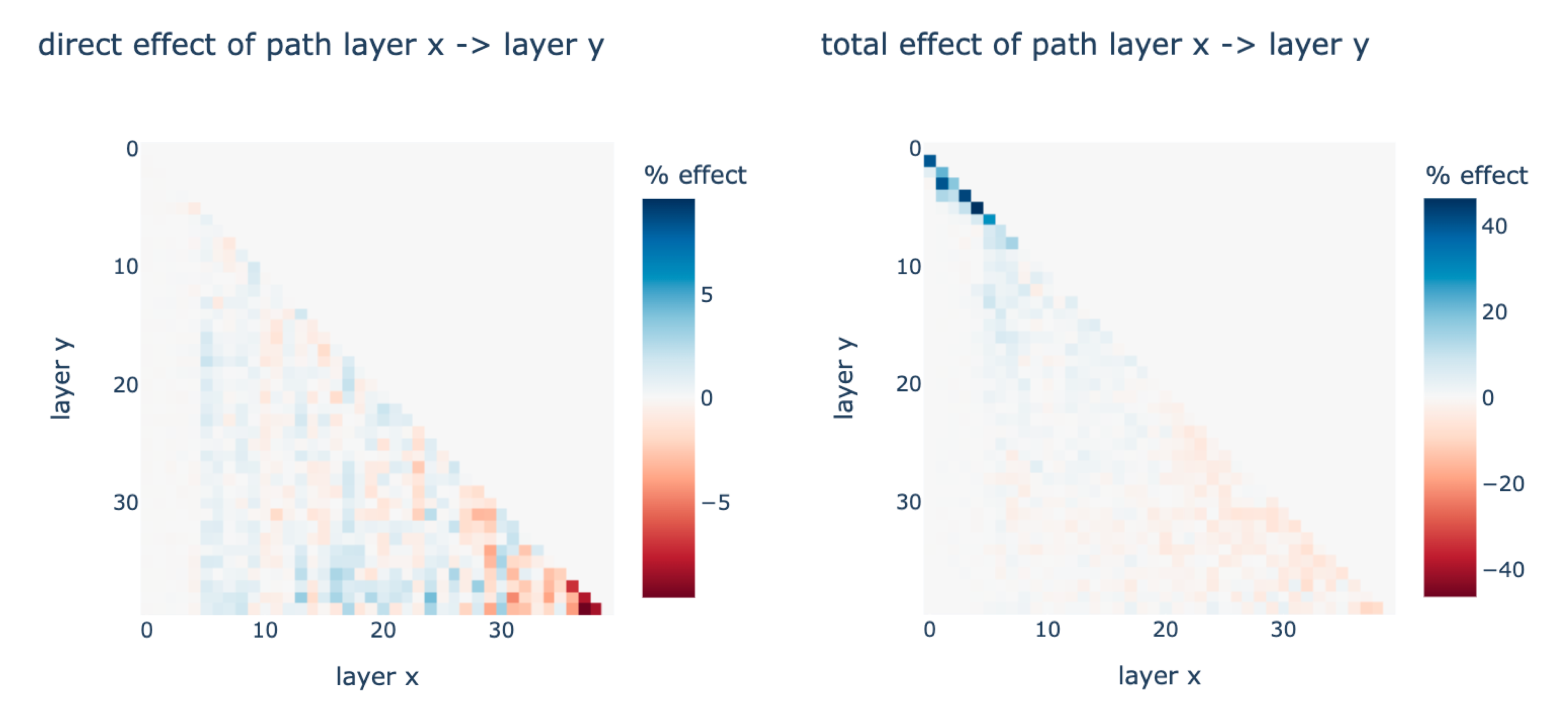
We also used path patching to measure the direct effect of the composition between every pair of layers on the output (left). At this point, we believe the answer to the question “how big is the circuit” to be: It’s pretty small, but not small enough. Although many parts of the model clearly don’t have any effect on the behavior, at 40 layers and 256 channels per layer, Leela Zero is a big model. If the goal is to provide a subgraph of the computation graph that captures the effect at the level of layer-channel pairs, it means to identify a subgraph on 40 * 256 = 10,240 nodes. Previous attempts at producing subgraphs of computations were all on a much smaller scale. The IOI work identified the biggest circuit to-date, a subgraph of GPT-2 at the level of attention heads and MLPs, and there are only a total of 12 * 13 = 156 nodes. Even though with techniques such as iterative path patching, it is possible to find an important subgraph for the behavior, we decided that it is not computationally tractable to produce such a a subgraph—nor would it be that interesting to have a subgraph that is nonetheless enormous and not semantically meaningful.

… but has a small, early bottleneck

This does not mean that we have nothing else to say about the this behavior, however. We also used path patching to measure the total effect of the composition between every pair of layers (right). This immediately reveals an important pattern: the first 5 or so layers function very differently from the rest of the model, and their computations have a very large effect on the output. This suggests the big picture that the first five layers are producing features that are then used by later layers in their computation of the final output.

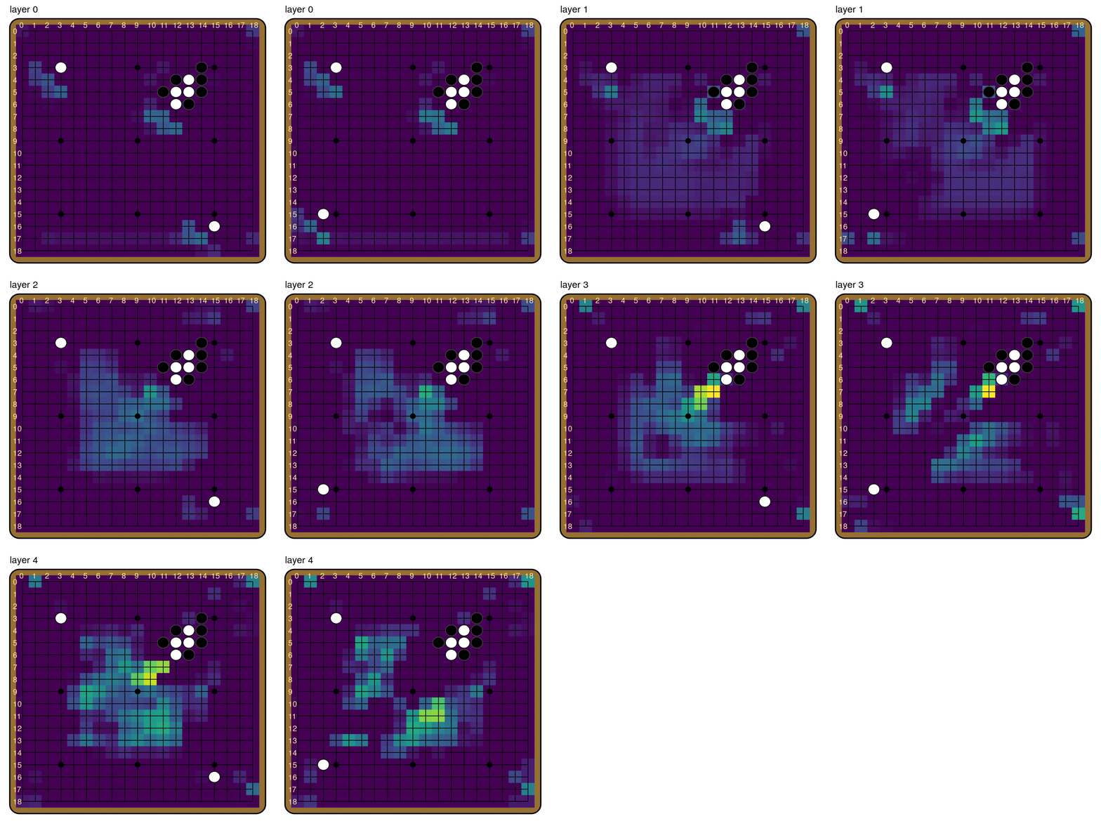
So is it possible to isolate some “breaker indicator” features in these early layers? It turns out that there is pretty much a single channel that encodes the model’s judgement of the ladder, channel 118. We find that simply patching the activations of channel 118 in layers 0-4 has an effect of 79.9% on the ladder reading! It is also the only channel that has such a large effect size when patched this way; the runner-up is channel 244, with an effect of 15.7% when patched in layers 0-4.

The fact that patching channel 118 in the first five layers has such a large effect is remarkable. By editing only 5 * 19 * 19 = 1,805 numbers in a forward pass, we essentially flip the model’s judgement on the ladder entirely. Although the pathway of information flow is very distributed in the rest of the model, it goes through a remarkably narrow, early bottleneck. The model pretty much records its judgement of the ladder in a single feature.

This also suggests that the reading of the ladder forms very early in the model. This is particularly interesting because in CNNs, there is a finite speed of information propagation, constrained by the receptive field of each neuron, which is in turn determined by the filter size. Since Leela Zero has two 3x3 convolutions per layer (i.e. per residual block), information can travel at most by 2 pixels per layer in each direction.^[12] For example, in the example board above, it takes at least 4 layers for the information at the location of the breaker to have any effect on the ladder move at all. And what we find is that the model essentially figures out the goodness of the ladder move as soon as it is possible to do so.

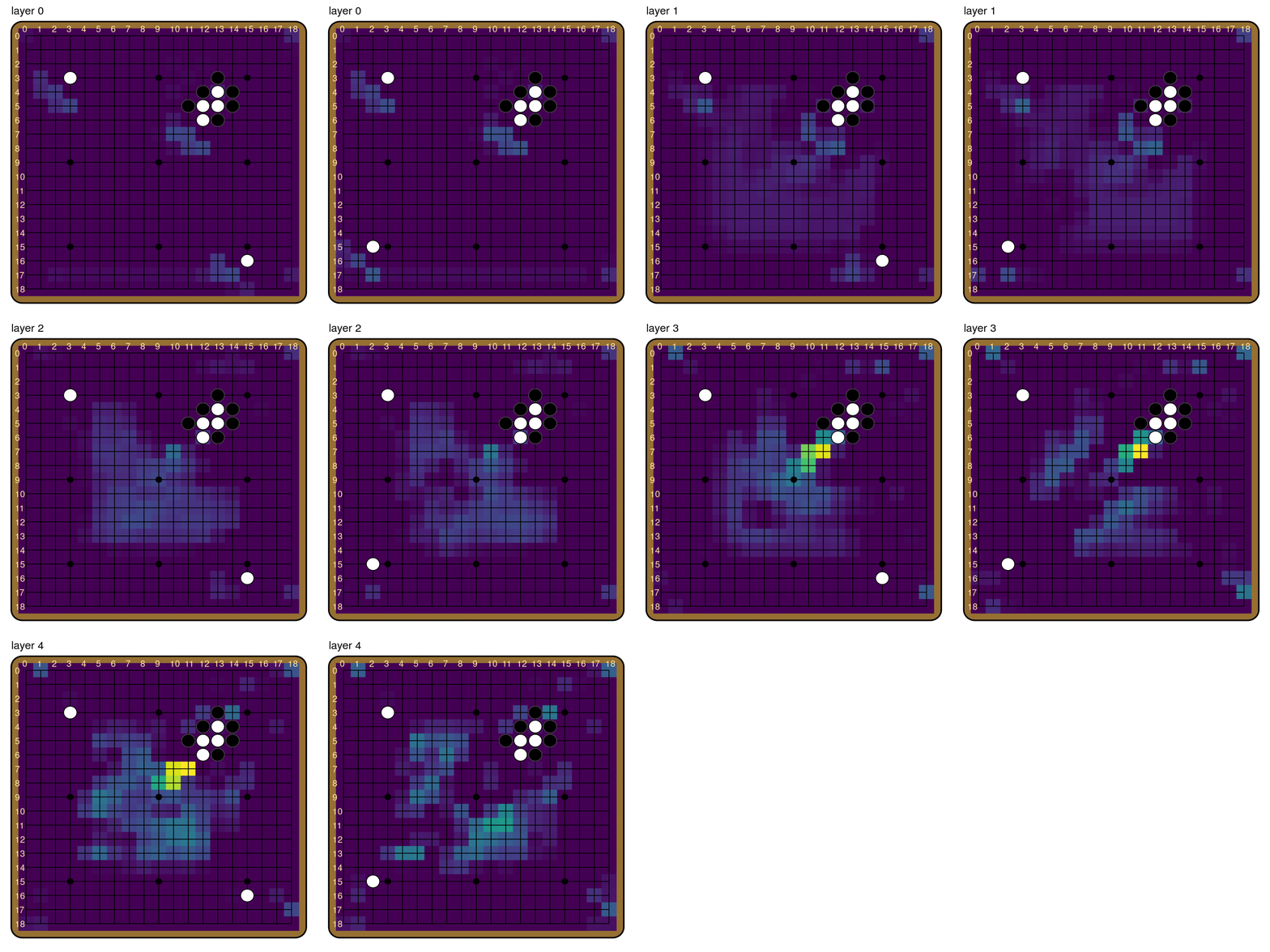
The breaker indicator feature, channel 118, in layers 0 through 4. The activations diverge drastically for the board with a ladder breaker and the one without by layer 4.

There are still many aspects of ladder reading that we do not understand. For example, how is the feature in channel 118 formed? Using iterative path patching, we identified 154 layer-channel pairs that are important for the formation of the breaker indicator. In particular, there are 41 channels in layer 0, 58 channels in layer 1, 37 channels in layer 2, and 18 channels in layer 3, for a total of 89 unique channels across the layers. The subgraph formed by these results in a 31.5% recovery of the ladder reading, or about 40% of the 79.9% effect of patching all paths to the breaker indicator. These numbers are not pretty, and further demonstrate the distributed nature of this behavior.

Breaker indicator ≠ ladder detector

There is also the question that how the model recognizes the start of a ladder in the first place. Note that the question we set out to answer is “given that there is a ladder, how does the model detect whether there is a ladder breaker?”, whose answer does not need to explain how the model recognizes ladders. Nonetheless, it is an interesting and important question. We found that although visually suggestive, channel 118 does not necessarily have anything to do with ladders, as its behavior does not depend on there being an actual ladder on the board. For example, if we moved one of the black stones, and the board no longer has a ladder, the policy output changes completely. However, activations in channel 118 appears near identical as in the ladder case.

Finally, recall that we have specialized to a particular ladder orientation, and one might wonder if the mechanism described here applies to the other orientations. From Naomi and Oliver’s REMIX project, it appears that the other ladder orientations each have a similar breaker indicator feature, similarly early in the model, that has a large effect on the ladder reading.

Conclusion and future work

To close, a few comments about the general takeaways from this project:

• I was pleasantly surprised many times along the way how easy it was to make progress understanding Leela Zero. This experience updated me more positively towards the feasibility of interpreting larger, more capable models.
• Much of our finding seems to suggest that the model is not making efficient use of its parameters. For example, the policy head ends up pretty much implementing the identity function, and the model figures out a lot of stuff by layer 4. The computer Go community is already moving towards wider and shallower models, and this work provides some evidence for the move.
• One question we were particularly interested in going into the project is to see if Leela Zero exhibits any signs of conducting internal search. In fact, we spotted a few channels that looked like they are playing out the ladder if we plotted their activations! But ultimately, we found those channels to not be causally relevant for the behavior. With the result that the ladder judgement is formed by layer 4, it seems that Leela Zero is using simple heuristics to read ladders, and not conducting internal search.

Below we list some future directions for this work:

• Is it possible to apply some other interpretability methods such as nonnegative matrix factorization (NMF) to analyze the weights, especially for the breaker indicator channel? The structure of the ResBlocks (with batch normalizations and ReLUs) poses some challenge for the naive method.
• Look into earlier training checkpoints and/or smaller versions of Leela Zero, see if the results presented here generalize at all. It’s known that Leela Zero could not read ladders at all a few years ago. Is it possible to find the point at which the model gained this capability via interpretability methods?
• Techniques used in this work can be easily applied to study other algorithmic tasks in Go [LW · GW], or even other games and other machine learning domains. A particularly interesting application would be to understand Wang et al (2022)’s adversarial policies against KataGo. For example, one of the adversarial policies essentially amounts to confusing the model about the number of liberties that a large circular group has, and capturing it “without the model noticing”. This attack somewhat transfers to Leela Zero as well. Can we find a mechanism for liberty-counting that explains the success of this attack?

Acknowledgement

This work was done during my internship at Redwood Research. Thanks in particular to: Buck Shlegeris, for encouraging me to pursue a Go interpretability project; Peter Schmidt-Nielsen, for teaching me Go and suggesting ladders as a behavior to study; Jesse Liptrap, for suggesting ideas for algorithmic tasks in Go; Arthur Conmy for the idea of residualification; Lawrence Chan, Arthur Conmy, Jeremy Côté, Xander Davies, Shiyue Li, Chris MacLeod, Peter Schmidt-Nielsen, Buck Shlegeris, and Alexandre Variengien for giving feedback on the draft. Many thanks also to REMIX residents Naomi Bashkansky, Hans Gundlach, Oliver Hayman, and Alok Singh for discussions and being great members of the Go Pod!

Citation information

Please cite this work as:

Haoxing Du, “Inside the mind of a superhuman Go model: How does Leela Zero read ladders?”, https://www.lesswrong.com/posts/FF8i6SLfKb4g7C4EL/inside-the-mind-of-a-superhuman-go-model-how-does-leela-zero (2023)

Appendix A: Details on policy head

Recall the architecture of the policy head, as shown above. Note that the convolutional layer here has 1x1 filters, which means that no actual spatial convolution is done, and this layer simply maps the 256 features at each pixel to 2 features. Let us call them feature0 and feature1. The investigation into the policy head was prompted by a look into these two features. For example, for the board below, this is what the two features look like.

They both look like the policy! However, they don’t quite have the same scale. Furthermore, feature0 is shifted down by a row compared to feature1 and the policy itself. That is, there is an extra row at the top, and the bottom row of the board is not present.

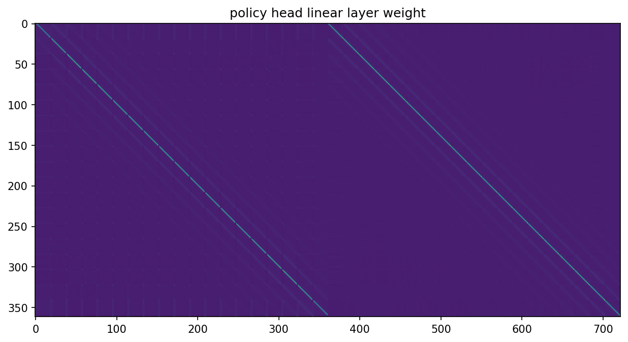
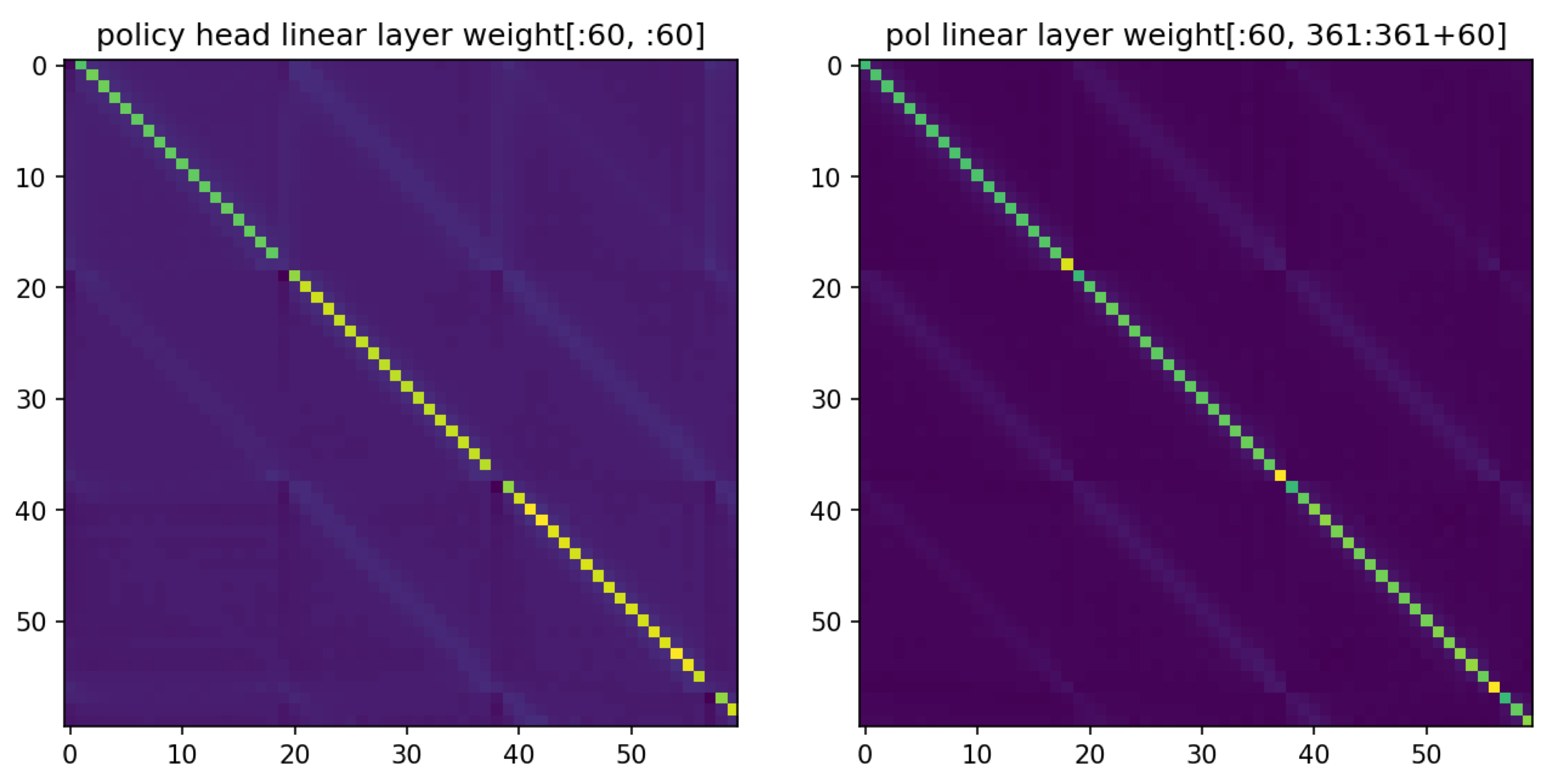
This must mean that the linear layer after this is pretty much an identity function (up to scaling). Indeed, if we plot the weight of the linear layer, it appears to be essentially two copies of the identity concatenated together. We see that in the part corresponding to feature0, it skips one column with a period of 19, as is required to restore the values to their real positions on the board.

Why is one of the features shifted, and what is the top row of the board used for? The answer lies in the last row of the linear layer’s weight: the weights for assembling the logit for the pass move (recall that the policy head outputs 19 * 19 + 1 = 362 values, with the last one being the pass logit). Rearranging the 722-dimensional weight array into their corresponding locations on the board across feature0 and feature1, we get the following:

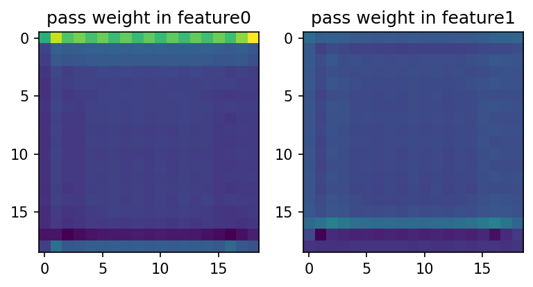
We see that the pass logit is mainly calculated from the first row of feature0, which explains why feature0 is shifted—so that the top row can be left to store global information about the pass move. We also see that feature1 also weakly contributes to the pass logit (the two images above have the same normalization), and that the third to last row of contributes more than anywhere else on the board. This led us to find the board that triples the pass probability described above [LW · GW].

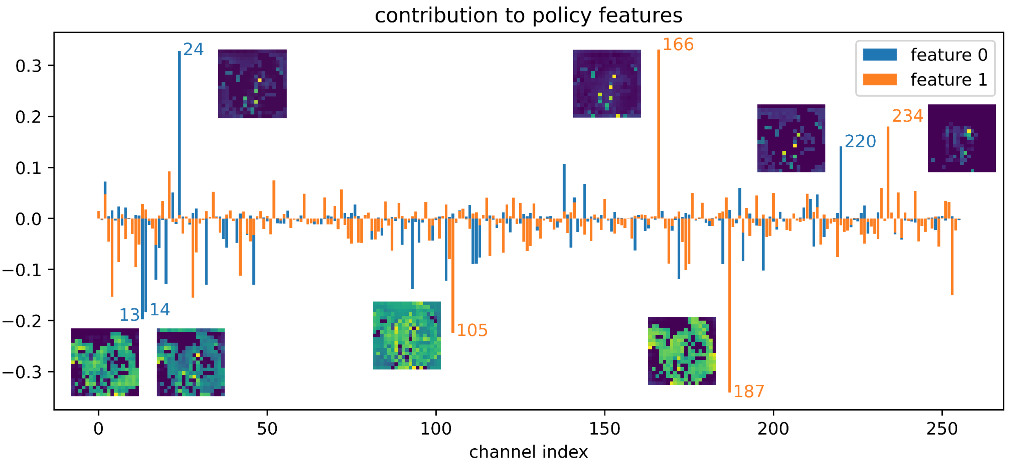
We could also go backwards from feature0 and feature1, and ask how they are formed. After all, they are each simply a linearly combination of the 256 features outputted by the residual tower. We can directly read off which of the 256 channels contribute most to each feature, by examining the weight of the convolutional layer, which is simply an array of dimension (256, 2). From this, we identify channel 24 as the greatest positive contributor to feature0, channel 166 as the greatest positive contributor to feature1. We see that the channels that contribute positively are those that highlight the top moves, and the channels that contribute negatively are those indicating the illegal moves. We also see that channels that contribute to feature0 are shifted by one row, as expected.

Appendix B: Details on value head

As a reminder, the architecture of the value head is shown above. Let us work backwards starting from the value output, and see what each layer is doing. The tanh serves to normalize the output to be in the range (-1, 1), and is monotonic. So the value pre-tanh is positive if the final value is positive, and negative if the final value is negative.

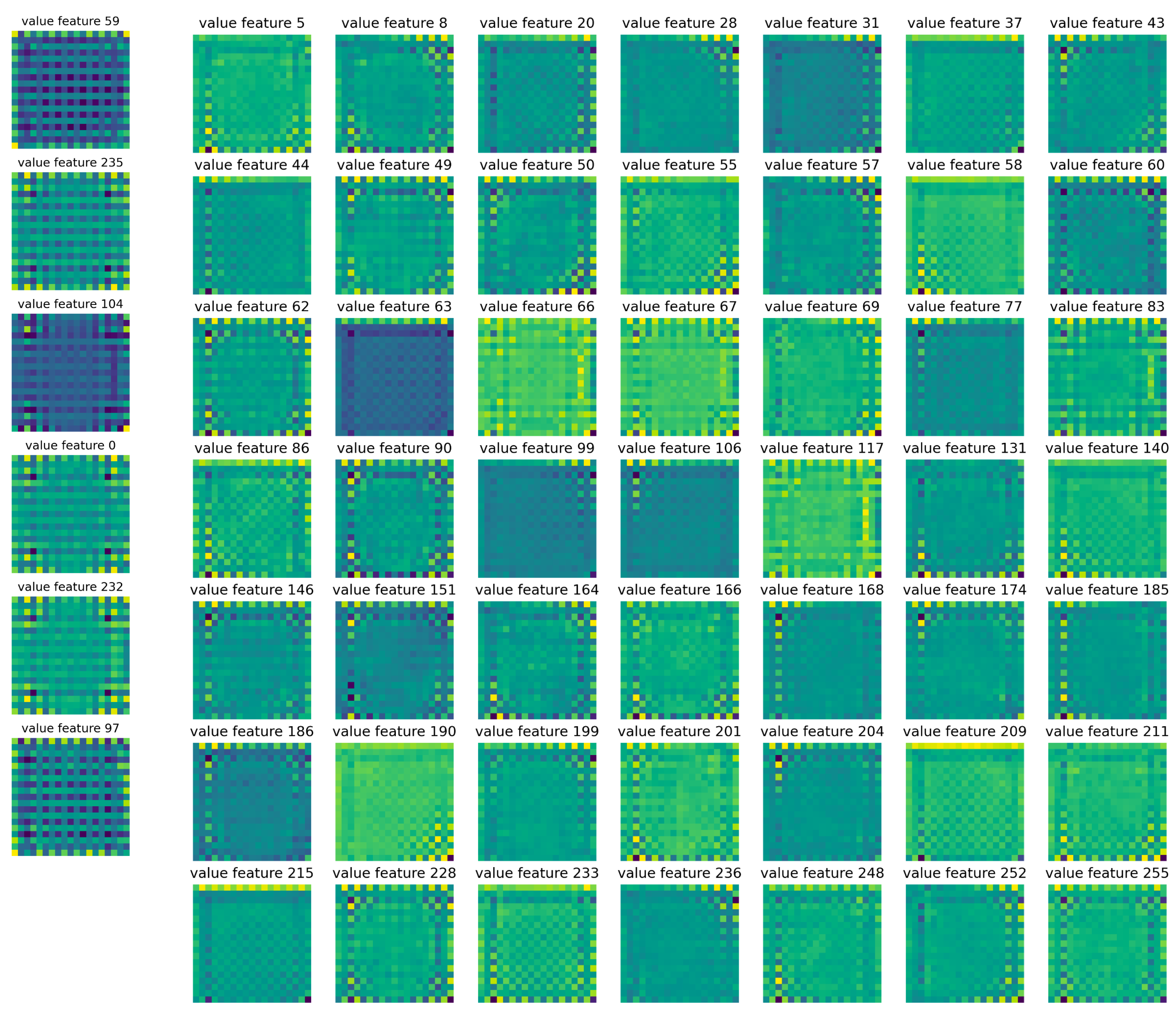
The pre-tanh value is computed by the second linear layer; that is, it’s a linear combination of the 256 features. We call these “value features”. Examining the weight of Linear 1, we see that only 6 of the value features contribute positively to the final value, and 49 of the value features contribute negatively. The other 201 weights are all less than 1e-7.

The value features are computed by Linear 0, from a single 19x19 feature. We call this the “value board”. So which parts of the board contribute to the positive value features, and which parts contribute to the negative ones? Here we exhibit contributions to all 6 positive features and all 49 negative features. We see that all of them have checkerboard patterns, and the positive and negative ones are offset. Summing the contributions within each category gives the images in the main text [LW · GW].

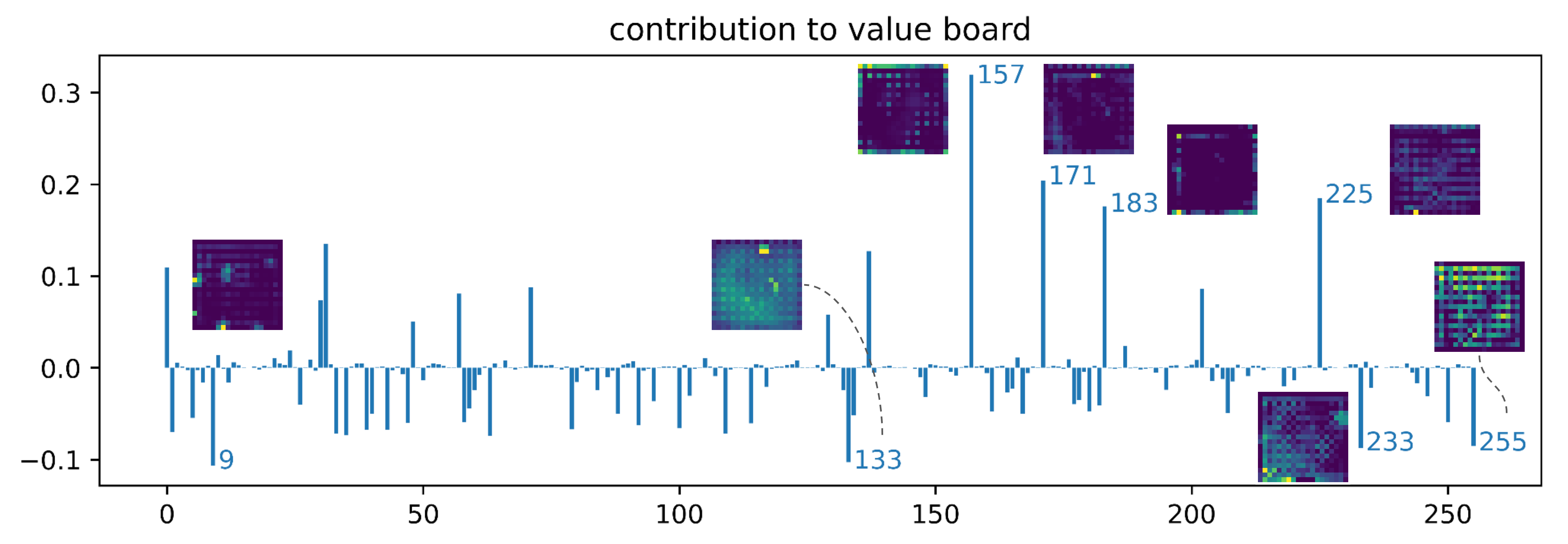
Lastly we can ask, how is the value board computed from the 256 channels outputted by the residual tower? Similar to the policy head, the residual tower output goes through a 1x1 convolution layer, and in this case gets combined into a single 19x19 value board. We again plot the weights directly, this time the 256-dimensional weight of the convolution layer. We see that the contributions are more distributed across the channels in this case (all the weights are greater than 1e-5), and identify a few of the channels that contribute the most. We again visualize the activations of top channels. These are with the same example board as above, which has a board value of -0.938 with white to play (i.e. black is almost certainly winning).

Appendix C: Algorithmic tasks in Go

This appendix contains a few other algorithmic tasks we identified. If you are interested in studying one of these, get in touch!

Identifying legal moves

In the AlphaZero algorithm, the policy head starts completely random, and is not given any information about the rules of the game. Nevertheless, the policy head learns to only put nonzero probabilities on legal moves. The only interaction between the policy head and the game rules is via MCTS, which sets the probability of illegal moves to zero, and the model must deduce the rule of not playing at illegal positions from data. How does the model figure out which moves are legal? It is perhaps not too hard for the model to realize that one never plays at already occupied intersection (and it would be nice to provide a mechanistic explanation for this as well), but much harder and more interesting to not violate ko rules and not play a suicide move.

Ko is the rule of Go that forbids moves that would result in a repeat of board positions. The policy of Leela Zero appears very good at avoiding simple ko situations. It is pretty easily checked that the feature planes at the $t-1$ time step are important for this behavior, but how is it implemented mechanistically?

Suicide moves are also interesting, because of the nonlocal reasoning required. Playing at an intersection with no liberty is forbidden, unless the play results in capture, and whether or not there is a capture might depend on board positions that are quite far away from the intersection in question. I have not tested this on Leela Zero and do not know how good it is at this behavior.

Escaping atari

REMIX residents Hans Gundlach and Alok Singh did some preliminary investigation into this behavior. When a group of stones is in atari (i.e. has only one liberty left), an obviously good move is to play at the remaining liberty to increase the group’s liberties. I think it makes sense to focus on the case where playing at the remaining liberty increases the number of liberties from 1 to 3, as increase from 1 to 2 is essentially the ladder case. This behavior feels particularly interesting as the shape of a group can be arbitrarily complicated, and the model has to have a general algorithm for detecting what is considered a group and counting its number of liberties. In fact, the recent adversarial policy against KataGo is essentially to make it confused about the number of liberties that a very large and meandering group has, and understanding the atari/liberty-counting algorithm might provide an explanation for why this attack works.

Counting territories

The value head judges the goodness of a board position. This is pretty nebulous in the early game, but in the end game it should be clear who is winning. Right before the game ends, the value of the board should come down to which player has more territory. Is the model calculating each player’s territory, and if so, how? I have not checked this behavior at all, but it should be possible to set up board positions such that moving a few stones flips the value head’s judgment entirely.

1. ^{^}

   Search refers to rolling out the game tree using Monte-Carlo Tree Search, aka “looking ahead”. For any given model, the more search it conducts the stronger it becomes. Also, this statement is now not completely true, see Wang et al's adversarial attack work.

2. ^{^}

   This is not quite accurate. Since the MCTS is rolled out using the policy head’s output, the policy head is in fact trained towards a fixed point of MCTS.

3. ^{^}

   A clarification on the confusing naming of DeepMind models: AlphaGo is the original Go model that first achieved superhuman performance. It introduced the architecture of a value network and a policy network, and used self-play to improve, but was initially trained on human data. Later came AlphaGo Zero which has the same design as AlphaGo, but used MCTS in self-play and was trained without any human input. Then came AlphaZero, which is the general algorithm that could be applied to basically any game, including chess and shogi.

4. ^{^}

   A more detailed explanation: The original AlphaGo Zero design has one feature plane that is all ones when black is to move, and all zeros when white is to move. When convolutions go past the edges of the board, with zero padding, it implicitly extends the feature plane with zeros in all directions. This means that when the feature plane is all ones, there is a boundary between on- and off-board, but when the feature plane is all zeros, there is none. In the orginal AlphaGo Zero design, black always gets the all-one feature and therefore some information about the size of the board, while white always gets the all-zero feature and no information; white still infers the board size, of course, by the fact that there are never stones placed outside of the board.

5. ^{^}

   To follow the content below you will likely need some familiarity with the rules of Go. If you don’t know the rules or need a refresher, see here for an introduction to Go.

6. ^{^}

   A caveat here: We in fact only used two possible starting lengths for the ladder, as we found that the judgement of the ladder is much worse for shorter and longer starting ladders. While it might appear surprising that the judgement is worse for longer ladders, we believe that it’s because ladders almost never get played out in real games of Go, and longer ladders are very rare in the training set.

7. ^{^}

   We also know from previous work that residual networks behave like ensembles of relatively shallow networks, and the effective paths in residual networks are relatively shallow. However, the type of residual network studied in Veit et al do not have nonlinearities between blocks, and is a “truer” residual network.

8. ^{^}

   This might seem obvious, but the model a priori has no reason to do this! In fact, this is a bit of a lie. We found that sometimes the model stores information about location (i, j) at the (i, j+1) position. See below [LW · GW].

9. ^{^}

   From looking at the activations of many channels across many boards, most channels show persistency for many layers at a time, if not throughout the whole model. Sometimes a channel gets reset partway through the model and changes role. Because of the ReLU applied to the residual stream at each layer, resetting just requires writing large negative numbers to the residual stream.

10. ^{^}

    Note that here I’m using the convention in computer vision that the origin is the top-left corner, and the first coordinate increases to the right, and the second coordinate increases to the bottom. This is unfortunately transposed from the convention for matrix entries—A[i, j] will show up at (j, i) on the board.

11. ^{^}

    One might wonder if the starting direction of the ladder matters as well, i.e. start with two horizontal stones vs two vertical ones. We found that this distinction doesn’t matter, which makes sense since in real games of Go, the start of a ladder can take many different shapes, and the important thing is its future trajectory.

12. ^{^}

    One might wonder if the starting direction of the ladder matters as well, i.e. start with two horizontal stones vs two vertical ones. We found that this distinction doesn’t matter, which makes sense since in real games of Go, the start of a ladder can take many different shapes, and the important thing is its future trajectory.

8 comments

Comments sorted by top scores.