A Correspondence Theorem

post by johnswentworth · 2020-10-26T23:28:06.305Z · LW · GW · 4 comments

Contents

    The Claim
    Key Ideas From The Math
    Applicability
    Conclusion
  Appendix: Proofs
    Correspondence Only If Independent Variation Subject to Deterministic Constraint
    Correspondence If Independent Variation Subject to Deterministic Constraint
None
4 comments

I’ve been thinking lately [LW · GW] about formalizations of the Correspondence Principle - the idea that new theories should reproduce old theories, at least in the places where the old theories work. Special relativity reduces to Galilean relativity at low speed/energy, general relativity reduces to Newtonian gravity when the fields are weak, quantum mechanics should reproduce classical mechanics at large scale, etc. More conceptually, it’s the idea that flowers are “real”: any model which does a sufficiently-good job of predicting the world around me should have some kind of structure in it corresponding to my notion of a flower (though it may not be ontologically basic).

I want theorems telling me when my models are of the right kind, and sufficiently-well-nailed-down, that I can expect some kind of correspondence along these lines to apply for any future theory (assuming the future theory has sufficiently strong predictive power). Ideally, this would allow us to take a model and extract the “generalizable” information from it, construct some universal representation of certain components of the model which lets us find the “corresponding” components in any other model with sufficiently-good predictive performance on the same data. (This problem [LW · GW] is one example of a potential application.)

This post introduces one such theorem. We’ll show that a (particular type of) correspondence theorem applies in exactly those cases where our model is able to make deterministic predictions about the relationship between some observable variables.

I've tried to keep the hairiest of the math in the appendices and the "key ideas from the math" section. If you want the key ideas with minimal math, then skip those sections.

The Claim

Here’s the setup. We have two random variables, $X_1$ and $X_2$, and we have enough data that we can perfectly figure out their joint distribution $P[X_1,X_2]$. We don’t necessarily know what physical process generates these variables - i.e. we don’t know the true underlying generative model. You can imagine some scientific experiment where we can collect lots of independent samples of $X_1,X_2$, then brute-force count how often each $(X_1,X_2)$ pair occurs in order to estimate $P[X_1,X_2]$, but we don’t have any way to experimentally probe the “internals” of the experimental setup. In other words, it's the traditional setup from frequentist probability.

We’ll assume that the class of “theories” we’re interested in are generative models - i.e. programs which take in some independent uniform variables and spit out $X_1,X_2$. For our purposes, we’ll assume these programs are represented as systems of circuits/causal DAGs/Bayes nets - see here [? · GW] for what that sort of representation looks like. (Note that this representation is Turing complete, so we’re not imposing any significant restriction.)

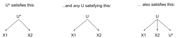
As long as $X_1$ and $X_2$ are not independent, any generative model which reproduces the distribution $P[X_1,X_2]$ must have some variable(s) upstream of both $X_1$ and $X_2$ - some common upstream cause(s) which account for the relationship between the variables. The claim I’d like to make is: any upstream variable(s) capable of accounting for the relationship between $X_1$ and $X_2$ must contain some “minimal” information. Formally: we can construct some variable $U^{\ast }$ (defined by the distributions $P\left[U^{\ast }\right],P\left[X_1|U^{\ast }\right],P\left[X_2|U^{\ast }\right]$) such that $X_1$ and $X_2$ are independent given $U^{\ast }$:

$P[X_1,X_2,U^{\ast }]=P\left[U^{\ast }\right]P\left[X_1|U^{\ast }\right]P\left[X_2|U^{\ast }\right]$

… and, for any other $U$ which induces conditional independence of $X_1$ and $X_2$, $U^{\ast }$ is a (possibly stochastic) function of $U$: for all $U$ such that 

$P[U,X_1,X_2]=P\left[U\right]P\left[X_1|U\right]P\left[X_2|U\right]$

... we have

$P[U,U^{\ast },X]=P\left[U\right]P\left[X|U\right]P\left[U^{\ast }|U\right]$.

Conceptually: $U^{\ast }$ is the “minimal” information about the relationship between $X_1$ and $X_2$. It must be “included in” any variable $U$ capable of accounting for the relationship between those two variables.

That’s the claim I’d like to make. However, that claim is too strong - not all distributions $P[X_1,X_2]$ have such a $U^{\ast }$. Indeed, in some sense “most” do not, though we can work around that to a large extent. The next section will explain exactly when we can construct such a $U^{\ast }$, and the appendix gives the proof. Specifically, we can construct $U^{\ast }$ in exactly those cases where the relationship between $X_1$ and $X_2$ is independent variation subject to a deterministic constraint. Formally: we can construct $U^{\ast }$ exactly when $P[X_1,X_2]$ can be represented as

$P[X_1,X_2]=I\left[f_1\right(X_1)=f_2(X_2\left)\right]P\left[f_1\right(X_1\left)\right]P\left[X_1|f_1\right(X_1\left)\right]P\left[X_2|f_2\right(X_2\left)\right]$

… for some deterministic functions $f_1,f_2$ (here $I[.]$ is the indicator function). In that case, we can choose $U^{\ast }=f_1\left(X_1\right)=f_2\left(X_2\right)$.

Key Ideas From The Math

We have to be able to calculate our “universal” upstream $U^{\ast }$ from any $U$ which induces independence of $X_1,X_2$. In particular, $X_1$ and $X_2$ are independent given either $X_1$ or $X_2$ itself - so we can choose either of those to be $U$. Combine that with the original requirements, and we have:

• $X_1$ independent of $X_2$ given $U^{\ast }$
• $U^{\ast }$ independent of $X_1$ given $X_2$
• $X_2$ independent of $U^{\ast }$ given $X_1$

This three-way conditional independence requirement is the main constraint which determines which distributions $P[X_1,X_2]$ have a $U^{\ast }$.

One easy way to satisfy this three-way conditional independence is when $X_1$, $X_2$, and $U^{\ast }$ are all just completely independent. Another is when all three are deterministically equal - i.e. $U^{\ast }=0$ implies $X_1=X_2=0$, $U^{\ast }=1$ implies $X_1=X_2=1$, etc. And of course we can rename variable values while maintaining three-way conditional independence - e.g. we could rename $X_1$ values from $[0,1,\dots ]$ to $[“fish”,12.38,\dots ]$. So all three variables isomorphic - rather than equal - also works: $U^{\ast }=f_1\left(X_1\right)=f_2\left(X_2\right)$, with $f_1$ and $f_2$ invertible.

We could also combine these two possibilities: $U^{\ast }$, $X_1$, and $X_2$ could each have two components, where one component is independent and the other component is fully determined by either of the other variables. For instance, we could have $U^{\ast }=(U^{\ast 1},U^{\ast 2})$, $X_1=(X_1^1,X_1^2)$, $X_2=(X_2^1,X_2^2)$, with $U^{\ast 1}$, $X_1^1$, and $X_2^1$ all completely independent, but $U^{\ast 2}$, $X_1^2$, and $X_2^2$ all deterministically isomorphic. Again, we can also rename variable values, so our variables don’t need to literally be written with two components.

… and that turns out to be the most general possibility.

Visually: if we lay out the distribution $P[X_1,X_2]$ in a matrix (with rows corresponding to $X_1$ values and columns corresponding to $X_2$ values), then we can arrange that matrix to look like this:

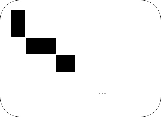
Here the dark blocks are nonzero values; everything else is zero. Within the dark blocks, we have $P[X_1,X_2]=P\left[X_1\right]P\left[X_2\right]$ - i.e. the dark blocks are each rank-1 submatrices. Intuitively, our distribution $P[X_1,X_2]$ consists of a deterministic relationship (the choice of which block we’re in) plus independent variation (choice of values within the block). This generalizes in the obvious way to the full distribution $P[U^{\ast },X_1,X_2]$: the full distribution consists of non-overlapping 3D blocks of nonzeros, with the three variables independent within each block.

For the full proof that these are the only distributions for which we can construct $U^{\ast }$, see the appendix.

Note that we do still have a degree of freedom in choosing $U^{\ast }$ - we can add or remove independent components. The obvious choice is to remove all the independent components from $U^{\ast }$, and just keep the deterministic component. Visually, we take $U^{\ast }$ to “choose a block” in the graphic above. (In fact, we could have just specified upfront that $U^{\ast }$ is a deterministic function of any possible $U$, rather than the more general stochastic function, but I usually prefer to use the more general version just in case the problem has some implicit embedded game with mixed equilibria - the stochastic function allows $U^{\ast }$ to “randomize its strategy”. In this case, it turns out that the generality doesn’t buy us anything, and that is itself useful to know; it means there’s probably no diagonalization shenanigans going on.)

The appendix proves that this choice of $U^{\ast }$ indeed satisfies all of our original conditions.

To wrap up this section, let’s write out the shape of $P[X_1,X_2]$ mathematically. Each value of $X_1$ has nonzero probability in only one “block”, so we can create a function $f_1\left(X_1\right)$ which picks out the block for each $X_1$ value. Likewise for $f_2\left(X_2\right)$. $P[X_1,X_2]$ can be nonzero only if $X_1$ and $X_2$ are in the same block: $f_1\left(X_1\right)=f_2\left(X_2\right)$. The chance of landing in a particular block is $P\left[f_1\right(X_1\left)\right]$ (which is equal to $P\left[f_2\right(X_2\left)\right]$, since $f_1\left(X_1\right)$ and $f_2\left(X_2\right)$ must always be equal). Within the block (i.e. conditional on $f_1\left(X_1\right)$), $X_1$ and $X_2$ are independent. Put all that together, and we get

$P[X_1,X_2]=I\left[f_1\right(X_1)=f_2(X_2\left)\right]P\left[f_1\right(X_1\left)\right]P\left[X_1|f_1\right(X_1\left)\right]P\left[X_2|f_2\right(X_2\left)\right]$

Since $f_1\left(X_1\right)$ picks out the block, and $U^{\ast }$ is the block choice, $U^{\ast }=f_1\left(X_1\right)=f_2\left(X_2\right)$. 

Applicability

At first glance, it looks like the conditions required to use this theorem are pretty restrictive. But there’s an easy trick to generalize it somewhat.

Suppose we have a distribution $P[X_1,X_2]$ which does not fully satisfy the requirements, but it does have a deterministic constraint: $g_1\left(X_1\right)=g_2\left(X_2\right)$ with probability 1. Then we can’t apply our correspondence theorem to $X_1$ and $X_2$, but we can apply it to $g_1\left(X_1\right)$ and $g_2\left(X_2\right)$. We can construct $U^{\ast }$ satisfying this:

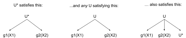
In particular, we can choose $U^{\ast }=g_1\left(X_1\right)=g_2\left(X_2\right)$.

So: whenever we can identify a deterministic constraint in the world, we can apply this correspondence theorem. In other words, deterministic constraints in one model should have corresponding structures in other models, to the extent that all models match the environment.

Note that “deterministic constraints” is exactly the content of most models in the hard sciences. For instance, equations in physics are almost always deterministic constraints on the trajectory of world-states. To the extent that these equations match the real world, we should see corresponding constraints in future theories/models which also match the real world.

We can push this further.

We haven’t talked about approximations here, but let’s assume that the theorem generalizes to approximations in the obvious way - i.e. approximately deterministic constraints give approximate correspondence, with independencies replaced by approximate independencies. Once we have approximations, we can construct deterministic constraints via statistical identification.

Here’s what that means. Consider something like the ideal gas law, $PV=nRT$. Observing a few specific particles will not tell us the pressure or temperature of the gas. Individual particles have only partial information about the high-level variables, so we don’t have a correspondence theorem. However, if we bucket together a whole bunch of particles, then we can get a very precise estimate of temperature and pressure - in stats terminology, $P$ and $T$ can be “identified” from our many independent particles. We can then have deterministic relationships between the identified variables, like $PV=nRT$. Then we can apply the correspondence theorem.

Similarly, we could identify variables using multiple “bunches of particles” - or, more generally, multiple meaurements/multiple lines of evidence. For instance, maybe we can use a whole bunch of measurements to determine the gravitational constant. If we do this again with another set of measurements, we expect to get the same number. That’s a deterministic constraint: gravitational constant calculated from one set of measurements should equal gravitational constant calculated from another. To the extent that this constraint matches the real world, our correspondence theorem says the gravitational constant should correspond to something in any future theory.

Conclusion

In some ways, this theorem leaves a lot to be desired. In particular, it assumes access to the “true distribution”, which I’d really like to get rid of. I expect there are other correspondence theorems to be found, with very different formulations, some of which would be better in that regard. For instance, for maximum entropy models, there’s an easy correspondence theorem which says “given an old model and a new model, either the constraints of the old model are satisfied by the new model, or we can construct a third model which strictly outperforms the new model”. (That theorem is unimpressive in other ways, however - it doesn’t really say anything about the “internal structure” of the models.)

Aside from direct use as a correspondence theorem, “independent variation subject to deterministic constraints” is an interesting thing to see pop out. It’s a common pattern in the sciences - it describes far-apart low-level variables in any abstraction [? · GW] where the high-level model is deterministic. I also think it’s equivalent to zero distributed information, which I previously predicted [? · GW] ought to show up quite often when looking at information relevant far away in a system. On top of that, humans often have a (mistaken) intuition that information works like sets - information comes in discrete chunks, and a variable either contains a chunk or it doesn’t. This leads to some common mistakes when studying information theory. For systems in which variation is independent subject to deterministic constraints, the “information is like sets” intuition is correct, and I suspect that it’s the only case where that picture works in general (for some formulation of “in general”).

It seems like there’s something fundamental about this pattern, and this correspondence theorem is another hint.

Appendix: Proofs

Even having guessed the answer, I found these proofs surprisingly difficult. There’s probably some way to set things up so it’s more obvious what to do, but I’m not sure what it is, other than that someone will tell me it has something to do with category theory.

The problem: we want $U^{\ast }$ for which

$P[U^{\ast },X_1,X_2]=P\left[U^{\ast }\right]P\left[X_1|U^{\ast }\right]P\left[X_2|U^{\ast }\right]$

and for all $U$ such that $P[U,X_1,X_2]=P\left[U\right]P\left[X_1|U\right]P\left[X_2|U\right]$, we have

$P[U,U^{\ast },X]=P\left[U\right]P\left[X|U\right]P\left[U^{\ast }|U\right]$.

We’ll show that:

• This is only possible when $P[X_1,X_2]=I\left[f_1\right(X_1)=f_2(X_2\left)\right]P\left[f_1\right(X_1\left)\right]P\left[X_1|f_1\right(X_1\left)\right]P\left[X_2|f_2\right(X_2\left)\right]$ for some $f_1,f_2$
• When $P[X_1,X_2]$ has that form, the choice $U^{\ast }=f_1\left(X_1\right)=f_2\left(X_2\right)$ works.

Correspondence Only If Independent Variation Subject to Deterministic Constraint

We'll start off the same as earlier: we want $U^{\ast }⫫X|U$ (in English: $U^{\ast }$ independent of $X$ given $U$) for any $U$ satisfying $X_1⫫X_2|U$. Well, there’s two choices for $U$ which definitely satisfy $X_1⫫X_2|U$: namely, $X_1$ and $X_2$ themselves. So:

• $X_1⫫U^{\ast }|X_2$
• $X_2⫫U^{\ast }|X_1$

… and by assumption, $X_1⫫X_2|U^{\ast }$. So, any two of the variables $X_1$, $X_2$, and $U^{\ast }$ are independent given the third.

Let’s write out $P[U,X_1,X_2]$ in two different ways, using two of our conditional independencies:

$P[U^{\ast },X_1,X_2]=P\left[X_1\right]P\left[X_2|X_1\right]P\left[U^{\ast }|X_1\right]=P\left[X_2\right]P\left[X_1|X_2\right]P\left[U^{\ast }|X_2\right]$

Note that $P\left[X_1\right]P\left[X_2|X_1\right]=P\left[X_2\right]P\left[X_1|X_2\right]=P[X_1,X_2]$, so we can cancel those terms out and find

$P\left[U^{\ast }|X_1\right]=P\left[U^{\ast }|X_2\right]$

… if $P[X_1,X_2]>0$. Note that, since our three-way independence condition is symmetric in the variables, we can also switch around the variables to get:

• $P\left[X_1|U^{\ast }\right]=P\left[X_1|X_2\right]$ when $P[U^{\ast },X_2]>0$
• $P\left[X_2|U^{\ast }\right]=P\left[X_2|X_1\right]$ when $P[U^{\ast },X_1]>0$

These are quite strong. Pick any two $X_2$ values, $x_2$ and $x_2^{\prime }$, for which any $x_1$ value has both $P[X_1=x_1,X_2=x_2]>0$ and $P[X_1=x_1,X_2=x_2^{\prime }]>0$. (Terminology: we’ll say that these two $X_2$ values “overlap” on $x_1$, i.e. either value occurs with nonzero probability when $X_1=x_1$. We'll also say that values of two different variables overlap when they have nonzero joint probability, e.g. $X_1=x_1$ overlaps $X_2=x_2$ iff $P[X_1=x_1,X_2=x_2]>0$). Then

$P[U^{\ast }|X_2=x_2]=P[U^{\ast }|X_1=x_1]=P[U^{\ast }|X_2=x_2^{\prime }]$

Furthermore, since $P[U^{\ast }|X_2=x_2]=P[U^{\ast }|X_2=x_2^{\prime }]$ for all $U^{\ast }$, any $U^{\ast }$ with $P[U^{\ast },X_2=x_2]>0$ will also have $P[U^{\ast },X_2=x_2^{\prime }]>0$. In other words, if two $X_2$ values overlap on any $X_1$ value, then they also overlap on all $U^{\ast }$ values which overlap either $X_2$ value. That, in turn, means

$P[X_1|X_2=x_2]=P[X_1|U^{\ast }=u^{\ast }]=P[X_1|X_2=x_2^{\prime }]$

… for any value $u^{\ast }$ on which $x_2,x_2^{\prime }$ overlap. Finally, this also means that two $X_2$ values which overlap on any $X_1$ value overlap on all $X_1$ values which overlap either $X_2$ value: ($P[X_1=x_1,X_2=x_2]>0$ and $P[X_1=x_1,X_2=x_2^{\prime }]>0$) for any $x_1$ implies that $P[X_1=x_1,X_2=x_2^{\prime }]>0$ on all $x_1$ with  $P[X_1=x_1,X_2=x_2]>0$, and vice versa.

That last condition is especially useful, since it means that overlap is transitive: if $x_2$ and $x_2^{\prime }$ overlap, and $x_2^{\prime }$ and $x_2^{\prime \prime }$ overlap, then $x_2$ and $x_2^{\prime \prime }$ overlap, and all three overlap on the same $X_1$ values.

That finally lets us construct our functions $f_1$ and $f_2$. Since we have transitivity of overlap, we can use overlap as an equivalence relation, and let $f_2\left(X_2\right)$ choose the equivalence class into which $X_2$ falls. $f_1\left(X_1\right)$ chooses the equivalence class of $X_2$ values with which $X_1$ overlaps (note that there can only be one, since this class contains all the $X_2$ values which overlap with this $X_1$ value). This is the “choice of block” from our earlier visual.

The rest follows (relatively) easily. From the definition of overlap, $P[X_1,X_2]=0$ whenever $f_1\left(X_1\right)\ne f_2\left(X_2\right)$. Our independence conditions from earlier give $P\left[X_1|X_2\right]=P\left[X_1|f_2\right(X_2\left)\right]$ (since all values in an overlap equivalence class give the same conditional distributions), so we have conditional independence given $f_2\left(X_2\right)$: 

$P[X_1,X_2|f_2(X_2\left)\right]=P\left[X_1|f_2\right(X_2\left)\right]P\left[X_2|f_2\right(X_2\left)\right]$

Then, we just expand:

$P[X_1,X_2]=P\left[f_2\right(X_2\left)\right]P[X_1,X_2|f_2(X_2\left)\right]=P\left[f_2\right(X_2\left)\right]P\left[X_1|f_2\right(X_2\left)\right]P\left[X_2|f_2\right(X_2\left)\right]$

Since $f_1\left(X_1\right)=f_2\left(X_2\right)$, we have

$P\left[X_1|f_2\right(X_2\left)\right]=I\left[f_1\right(X_1)=f_2(X_2\left)\right]P\left[X_1|f_1\right(X_1\left)\right]$

… which gives us our final expression:

$P[X_1,X_2]=I\left[f_1\right(X_1)=f_2(X_2\left)\right]P\left[f_2\right(X_2\left)\right]P\left[X_1|f_1\right(X_1\left)\right]P\left[X_2|f_2\right(X_2\left)\right]$

(And note that we can freely switch $P\left[f_2\right(X_2\left)\right]$ with $P\left[f_1\right(X_1\left)\right]$ here.)

One side note: I’ve defined $f_1$ and $f_2$ here as selecting equivalence classes, which is kind of annoying - it doesn’t give us a clean explicit representation. If we want an explicit representation, we can choose $f_1\left(X_1\right)=(x_2\to P[X_2=x_2|X_1\left]\right)$, and likewise for $f_2$. This leads to “fun” expressions like $P\left[X_1|\right(x_2\to P[X_2=x_2|X_1]\left)\right]$. See the Minimal Map [LW · GW] post for how to interpret expressions like that.

Correspondence If Independent Variation Subject to Deterministic Constraint

Now we assume that $P[X_1,X_2]$ has the right form, declare that $X_1$ and $X_2$ are independent given some $U$, and show that $f_1\left(X_1\right)$ (or equivalently, $f_2\left(X_2\right)$) is a function of $U$, implying that it’s independent of $X_1$ and $X_2$ given $U$.

Suppose that $f_1\left(X_1\right)$ is not a function of $U$ - i.e. there is some value $u$ of $U$ for which $f_1\left(X_1\right)$ could have two different values $f,f^{\prime }$ each with nonzero probability. Then, since $X_1$ and $X_2$ are independent given $U$:

$P[U=u,f_1(X_1)=f,f_2(X_2)=f^{\prime }]=$$P[U=u]P\left[f_1\right(X_1)=f|U=u]P\left[f_2\right(X_2)=f^{\prime }|U=u]$

Since $f_1\left(X_1\right)=f_2\left(X_2\right)$ with probability 1, we must have $P\left[f_2\right(X_2)=f^{\prime }|U=u]=P\left[f_1\right(X_1)=f^{\prime }|U=u]$. Substituting:

$P[U=u,f_1(X_1)=f,f_2(X_2)=f^{\prime }]=P[U=u]P\left[f_1\right(X_1)=f|U=u]P\left[f_1\right(X_1)=f^{\prime }|U=u]$

Now, by assumption:

• $f$ and $f^{\prime }$ are different
• $P\left[f_1\right(X_1)=f|U=u]$ and $P\left[f_1\right(X_1)=f^{\prime }|U=u]$ are both nonzero

… thus $P[U=u,f_1(X_1)=f,f_2(X_2)=f^{\prime }]>0$.

… but that’s a contradiction, because that means there’s a nonzero probability that $f_1\left(X_1\right)\ne f_2\left(X_2\right)$.

Thus, $f_1\left(X_1\right)$ is always a function of $U$, and is therefore independent of $X_1$ and $X_2$ (and anything else) given $U$.

4 comments

Comments sorted by top scores.