UML final

post by Rafael Harth (sil-ver) · 2020-03-08T20:43:58.897Z · LW · GW · 1 comments

Contents

  Multiclass Prediction
    Approach 1: Reduction to Binary Classification
    Approach 2: Linear Programming
    Approach 3: Surrogate Loss and Stochastic Gradient Descent
  Remaining Material
    Naive Bayes Classifier
    Feature Selection
    Regularization and Stability
    Generative Models
    Advanced Theory
  Closing Thoughts on the Book
None
1 comment

(This is the fourteenth and final post in a sequence on Machine Learning based on this book. Click here [? · GW] for part I.)

The first part of this post will be devoted to multiclass prediction, which is the last topic I'll cover in the usual style. (It's on the technical side; requires familiarity with a bunch of concepts covered in earlier posts.) Then follows a less detailed treatment of the remaining material and, finally, some musings on the textbook.

Multiclass Prediction

For this chapter, we're back in the realm of supervised learning.

Previously in this sequence, we've looked at binary classification (where $|Y|=2$) and regression (where $Y=R$). In multiclass prediction or multiclass categorization, we have $|Y|\in N$ but $|Y|>2$. For simplicity, we take the next simplest case, i.e., $|Y|=3$. (Going up from there is straight-forward.) More specifically, consider the problem of recognizing dogs and cats in pictures, which we can model by setting $Y=\{\text{dog},\text{cat},\text{noanimal}\}$. For the purposes of this chapter, we ignore the difficult question of how to represent the instance space $X$.

We take the following approach:

• train a function to compute a score for each label that indicates how well the instance fits that label
• classify each new domain point as the best-fitting label

In our case, this means we are interested in learning a function of the form $f:X\times Y\to R$. Then, if we have

$f(x,\text{cat})=2f(x,\text{dog})=\sqrt{5}f(x,\text{no\_animal})=-1$

this translates into something like "$x$ kinda looks like a dog, but a little bit more like a cat, and it does seem to be some animal." Each such function determines a predictor $h_f:X\to Y$ via the rule $h_f\left(x\right)={\text{argmax}}_{y\in Y}f(x,y)$.

We will restrict ourselves to linear predictors. I.e., we assume that the feature space $X$ is represented as something like $R^d$ and our predictors are based on hyperplanes.

With the setting established, the question is how to learn $f$.

Approach 1: Reduction to Binary Classification

Suppose (unrealistically) that $X=R^2$ and our training data looks like this:

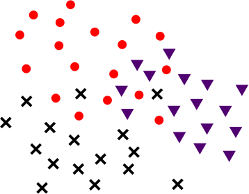
where

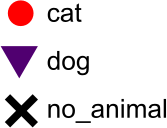
We could now train a separate scoring function for each label. Starting with cats, we would like a function $f_{\text{cat}}:X\to R$ that assigns each point a score based on how much it looks like a cat. For $f_{\text{cat}}$, the label $\text{cat}$ corresponds to the label 1, whereas $\text{dog}$ and $\text{no\_animal}$ both correspond to the label 0. In this setting, learning $f_{\text{cat}}$ corresponds to finding a passable hyperplane. (Apply linear programming for Soft Support Vector Machines. [LW · GW])

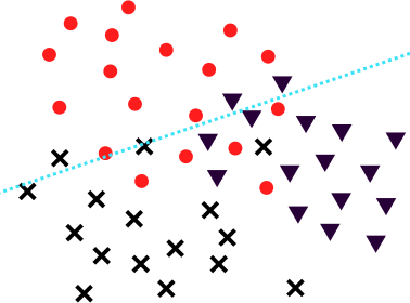
Note that, while hyperplanes are used to classify points, they do, in fact, produce a numerical score based on how far on the respective side each point is.

Next, we train a $f_{\text{dog}}$ function. Perhaps its hyperplane looks like so:

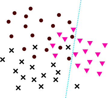
And, finally, a $f_{\text{no\_animal}}$ function in a similar fashion. Then, we define

$f(x,\text{cat}):=f_{\text{cat}}\left(x\right)\forall x\in X$

And likewise with $\text{dog}$ and $\text{no\_animal}$. As before, we let $h_f\left(x\right)\in {\text{argmax}}_{y\in Y}f(x,y)$.

Note that a point might be classified correctly, even if it is on the wrong side of the respective hyperplane. For example, consider this point:

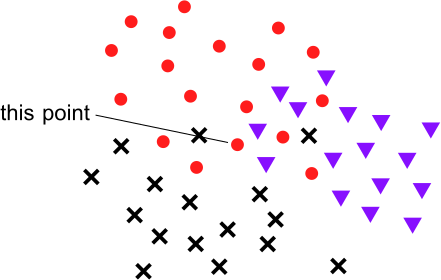
$f_{\text{cat}}$ thought this point was not a cat, but it thought it less intensely than $f_{\text{dog}}$ thought that it was not a dog. Thus, depending on $f_{\text{no\_animal}}$'s verdict, the $\text{argmax}$ that $h$ computes might still put out a cat label. Of course, the reverse is also true – a point might be classified as a cat by $f_{\text{cat}}$ but also as a dog by $f_{\text{dog}}$, and if the dog classification is more confident, the $\text{argmax}$ will pick that as the label.

The reduction approach is also possible with predictors that merely put out a binary yes/no. However, numerical scores are preferable, precisely because of cases like the above. If we had used classifiers only, then $h_{\text{cat}}\left(x\right)=h_{\text{dog}}\left(x\right)=h_{\text{no\_animal}}\left(x\right)=0$ for $x=\text{this point}$ and we could do no better than to guess.

While the reduction approach can work, it won't have the best performance in practice, so we look for alternatives.

Approach 2: Linear Programming

Using the fact that we are in the linear setting, we can rephrase our problem as follows: let $\text{cat}=0,\text{dog = 1},\text{no\_animal}=2$, then we wish to find three vectors $w_0,w_1,w_2$ such that, for all training points $(x,i)$, we have $⟨w_i,x⟩>⟨w_j,x⟩$ for all $j\ne i$. In words: for each training point, the inner product with the vector measuring the similarity to the correct label needs to be larger than the inner product with the other vectors (in this case, the 2 others). This can be phrased as a linear program in much the same way as for Support Vector Machines (post VIII [LW · GW]).

However, it only works if such vectors exist. In practice, this is only going to be the case if the dimension is extremely large.

Approach 3: Surrogate Loss and Stochastic Gradient Descent

A general trick I first mentioned in post V [LW · GW] is to apply Stochastic Gradient Descent (post VI [LW · GW]) with respect to a surrogate loss function (i.e., a loss function that is convex and upper-bounds the first loss). In more detail (but still only sketched), this means we

• represent the class of hypotheses $H$ as a familiar set (easy for hyperplanes)
• for each labeled data point $(x_i,y_i)$ in our training sequence $S$, construct the point-based loss function ${\ell }_{(x_i,y_i)}:H\to R$
• construct convex point-based loss functions ${\ell }_{(x_i,y_i)}^{\ast }:H\to R$ such that ${\ell }_{(x_i,y_i)}\le {\ell }_{(x_i,y_i)}^{\ast }$
• compute the gradients $\nabla {\ell }_{(x_i,y_i)}^{\ast }\left(h\right)$ and update our hypothesis step by step, i.e., set $h^{(t+1)}:=h^{\left(t\right)}-\eta \nabla {\ell }_{(x_t,y_t)}\left(h^{\left(t\right)}\right)$.

To do this, we have to change the framing somewhat. Rather than measuring the loss of our function $f:X\times Y\to R$ (or of the predictor $h_f:X\to Y$), we would like to analyze the loss of a vector $w\in R^n$ for some $n\in N$. However, we do not want to change our high-level approach: we still wish to evaluate all pairs $(x,\text{cat})$ and $(x,\text{dog})$ and $(x,\text{no\_animal})$ separately.

This can be done by the following construction. Let $d$ be the number of coordinates that we use for each label, i.e., $X=R^d$. We can "expand" this space to $R^{3d}$ and consider it to hold three copies of each data point. Formally, we define the function $\Psi :X\times Y\to R^{3d}$ by $\Psi (x,\text{cat})=x\circ 0\circ 0$ and $\Psi (x,\text{dog})=0\circ x\circ 0$ and $\Psi (x,\text{no\_animal})=0\circ 0\circ x$, where $0$ is the vector consisting of $d$ many zeros. Then we can represent all parts of our function $f$ as a single vector $w\in R^{3d}$. If we take the inner product $⟨\Psi (x,\text{dog}),w⟩$, it will only apply the part of $w$ that deals with the dog label since the other parts of $\Psi (x,\text{dog})$ are all 0s.

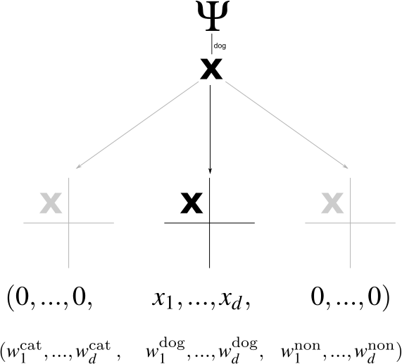
Thus, what was previously $f(x,\text{cat})$ is now $⟨\Psi (x,\text{cat}),w⟩$. The nontrivial information that was previously encoded in $f$ is now encoded in $w$. Our predictor $h_w$ (which is fully determined by $w$) follows the rule $h_w\left(x\right)\in {\text{argmax}}_{y\in Y}⟨\Psi (x,y),w⟩$. Thus, we still assign to each point the label for which it received the highest score. Note that $w$ makes use of all $3d$ coordinates; there's no repetition.

Now we need to define loss functions. Since our goal is to apply Stochastic Gradient Descent, we focus on point-based loss functions ${\ell }_{(x,y)}$ that measure the performance of $w$ on the point $(x,y)$ only. (We write $x$ fat now since we specified that it's a vector.) One possible choice is the generalized 0-1 loss, ${\ell }_{(x,y)}^{\text{gen-0-1}}\left(w\right)=1_{h_w\left(x\right)\ne y}$ that is 1 iff $w$ assigns the wrong label and 0 otherwise. However, this choice may not be optimal: if an image contains a cat, we probably prefer the predictor claiming it contains a dog to it claiming it doesn't contain any animal. Therefore, we might wish to define a function $L:Y\times Y\to R$ that measures how different two labels are. Then, we set ${\ell }_{(x,y)}^L\left(w\right):=L\left(h_w\right(x),y)$. The function $L$ should by symmetric and non-negative, and it should be the case that $L(y,y)=0\forall y\in Y$. For our example, a reasonable choice could be

$\begin{array}{cccccc}L(\text{cat},\text{cat})& =0& L(\text{cat},\text{dog})& =0.2& L(\text{cat},\text{no\_animal})& =1\\ L(\text{dog},\text{cat})& =0.2& L(\text{dog},\text{dog})& =0& L(\text{dog},\text{no\_animal})& =1\\ L(\text{no\_animal},\text{cat})& =1& L(\text{no\_animal},\text{dog})& =1& L(\text{no\_animal},\text{no\_animal})& =0\end{array}$

The loss function ${\ell }_{(x,y)}^L$ as defined above is non-convex: if $h_w$ and $h_{w^{\prime }}$ output different labels on $x$, they will have different losses, which means that somewhere on the straight line between $w$ and $w^{\prime }$, the loss ${\ell }_{(x,y)}^L$ makes a sudden jump (and sudden jumps make a function non-convex [LW · GW]). Thus, our goal now is to construct a convex loss function ${\ell }^{\ast }$ such that, for each $(x,y)$ in the training sequence, ${\ell }_{(x,y)}^{\ast }$ upper-bounds ${\ell }_{(x,y)}^L$.

To this end, consider the term

$⟨w,\Psi (x,h_w(x\left)\right)⟩-⟨w,\Psi (x,y)⟩$

for any point $(x,y)$. Recall that the predictor $h_w$ chooses its label precisely in such a way that the above inner product is maximized. It follows that the term above is non-negative. (It's 0 for $y=h_w\left(x\right)$). Therefore, adding this term to our loss will upper-bond the original loss. We obtain

$L\left(h_w\right(x),y)+(⟨w,\Psi (x,h_w(x\left)\right)⟩-⟨w,\Psi (x,y)⟩)$

This term penalizes $w$ for (1) the difference between the predicted and the correct label; and (2) the difference between $w$'s score for the predicted and the correct label. This would be a questionable improvement – we now punish $w$ twice for essentially the same mistake. But the term above is only an intermediate step. Now, instead of using $h_w$ in the term above, we can take the maximum over all possible labels $y^{\prime }\in Y$; clearly, this will not make the term any smaller. The resulting term will define our loss function. I.e.:

${\ell }_{(x,y)}^{\ast }\left(w\right):=\underset{y^{\prime }\in Y}{max}(L(y^{\prime },y)+(⟨w,\Psi (x,y^{\prime })⟩-⟨w,\Psi (x,y)⟩))$

Note that, unlike before, the difference between the two inner products may be negative.

Let's think about what these two equations mean (referring two the two centered equations, let's call them E1 and E2). E1 (the former) punishes $w$ in terms of the correct label $y$ and the label which $w$ guessed: it looks both at how far its prediction is off and how wrong the label is. E2 does the same for $y^{\prime }=h_w\left(x\right)$, so it will always put out at least as high of an error. However, E2 also looks at all the other labels. To illustrate the effect of this, suppose that the correct label $y$ is $\text{dog}$, but $h_w$ guessed $\text{cat}$. The comparison of the correct label $\text{dog}$ to the guessed label $\text{cat}$ (corresponding to $y^{\prime }=\text{cat}$) will yield an error of 0.2 (for the difference between both labels) plus the difference between $w$'s score for both (which is inevitably positive since it guessed $\text{cat}$). Let's say $⟨w,\Psi (x,\text{cat})⟩=0.8$ and $⟨w,\Psi (x,\text{dog})⟩=0.5$, then the difference is another 0.3 and the total error comes out $0.5$.

Now consider the term for $y^{\prime }=\text{no\_amimal}$. Suppose $⟨w,\Psi (x,\text{no\_animal})⟩=0.3$; in that case, $w$ did think $\text{dog}$ was a more likely label than $\text{no\_animal}$, but only by 0.2. Therefore, $⟨w,y^{\prime }⟩-⟨x,y⟩=-0.2$. This is a negative term, which means it will be subtracted from the error. However, the loss function "expects" a difference of 1, because that's the difference between the labels $\text{dog}$ and $\text{no\_animal}$. Thus, the full term $L(y^{\prime },y)+(⟨w,y^{\prime }⟩-⟨x,y⟩)$ for $y^{\prime }=\text{no\_animal}$ comes out at $1-0.2=0.8$, which is higher than for $\text{cat}$.

(Meanwhile, the trivial case of $y^{\prime }=\text{dog}$ – i.e., comparing the correct label to itself – always yields an error of 0.)

Alas, the loss function ends up scolding $w$ the most not for the (slightly) wrong label it actually put out, but for the (very) wrong label it almost put out. This might be reasonable behavior, although it certainly requires that the numerical scores are meaningful. In any case, note that the primary point of formulating the point-based loss functions ${\ell }_{(x,y)}^{\ast }$ was to have it be convex, so even if the resulting function were less meaningful, this might be an acceptable price to pay. (To see that it is, in fact, convex, simply note that it is the maximum of a set of linear functions.)

With this loss function constructed, applying Stochastic Gradient Descent is easy. We start with some random weight vector $w^{\left(0\right)}$. At step $t$, we take $w^{\left(t\right)}$ and the labeled training point $(x_t,y_t)$. Consider the term

${\ell }_{(x_t,y_t)}^{\ast }\left(w^{\left(t\right)}\right):=\underset{y^{\prime }\in Y}{max}(L(y^{\prime },y_t)+(⟨w^{\left(t\right)},\Psi (x_t,y^{\prime })⟩-⟨w^{\left(t\right)},\Psi (x_t,y_t)⟩))$

The gradient of the maximum of a bunch of functions is the maximum of their gradients. Thus, if $y^{\ast }$ is the label for which the above is maximal, then

$\nabla {\ell }_{(x_t,y_t)}^{\ast }\left(w^{\left(t\right)}\right)=\Psi (x_t,y^{\ast })-\Psi (x_t,y_t)$

Therefore, our update rule is $w^{(t+1)}:=w^{\left(t\right)}-\eta \left[\Psi \right(x_t,y^{\ast })-\Psi (x_t,y_t\left)\right]$.

Remaining Material

Now we get to the stuff that I read at least partially but decided to cover in less detail.

Naive Bayes Classifier

Naive Bayes is a simple type of classifier that can be used for specific categorization tasks (supervised learning), both binary classification and multi-classification but not regression. The "naive" does not imply that Bayes is naive; instead, it is naive and uses Bayes' rule.

We usually frame our goal in terms of wanting to learn a function $h:X\to Y$. However, we can alternatively ask to learn the conditional probability distribution $D\left(\right(x,y\left)|x\right)$. If we know this probability – i.e., the probability of observing a (point, label) pair once we see the point – it is easy to predict new points.

For the rest of this section, we'll write "probability" as $Pr$ rather than $D$, and we'll write $Pr\left(y|x\right)$ rather than $Pr\left(\right(x,y\left)|x\right)$.

Now. For any pair $(x,y)\in X\times Y$, we can express $Pr\left(y|x\right)$ in terms of $Pr\left(x|y\right)$ and $P\left(x\right)$ and $P\left(y\right)$ using Bayes' rule. This implies that knowing all the $Pr\left(x|y\right)$ is sufficient to estimate any $Pr\left(y|x\right)$ (the priors on $x$ and $y$ are generally not an issue). The difficulty is that $X$ is usually infinite and we only have access to some finite training sequence $S$.

For this reason, Naive Bayes will only be applicable to certain types of problems. One of them, which will be our running example, is document classification in the bag of words model. Here, $X=\{0,1{\}}^d$ where $d$ is the number of words in our dictionary, and each document is represented as a vector $x=(x_1,...,x_d)\in X$. where bit $x_i$ indicates whether or not the $i$-th word of our dictionary appears in [the document represented by $x$]. Thus, we throw away order and repetitions but keep everything else. Furthermore, $Y$ is a set of possible topics, and the goal is to learn a predictor that sees a new document and assigns it a topic.

The crucial property of this example is that each coordinate of our vectors is very simple. On the other hand, the vectors themselves are not simple: we have $d\approx 170.000$ (number of words in the dictionary), which means we have about $2^{170000}$ parameters to learn (all $P\left(y|x\right)$). The solution is the "naive" part: we assume that all feature coordinates are independent so that $Pr\left(\right(x_1,...,x_d\left)|y\right)={\prod }_{i=1}^{d}Pr\left(x_i|y\right)$. This assumption is, of course, incorrect: the probabilities for $x_i=\text{"football"}$ and $x_j=\text{"goal"}$ are certainly not independent. But an imperfect model can still make reasonable predictions.

Thus, naive Bayes works by estimating the parameters $Pr\left(x_i|y\right)$ for any $i\in \left[d\right]$ and $y\in Y$. If $Y$ consists of 100 possible topics, then we wish to estimate $100\cdot d\approx \mathrm{17.000.000}$ parameters, which may be feasible.

Given a labeled document collection (the training sequence $S$), estimating these parameters is now both simple and fast, which is the major strength of Naive Bayes. In fact, it is the fastest possible predictor in the sense that each training point only has to be checked once. Note that $Pr\left(x_i|y\right)$ is the probability of encountering word $x_i$ in a document about topic $y$. For example, it could be the probability of encountering the word "Deipnophobia" (fear of dinner parties) in a document about sports. To estimate this probability, we read through all documents about sport in our collection and keep track of how many of them contain this term (spoilers: it's zero). On that basis, we estimate that

$Pr\left(\text{"Deipnophobia"}|\text{sport}\right)=\frac{|\left\{\text{documents about sport with this word}\right\}|+1}{|\left\{\text{documents about sport}\right\}|+1}=\frac{1}{1532}$

Why the $+1$? Well, as this example illustrates, the natural estimate will often be 0. However, a 0 as our estimate will mean that any document which contains this word has no chance to be classified as a sports document (see equations below), which seems overkill. Hence we "smooth" the estimate by the $+1$.

Small tangent: I think it's worth thinking about why this problem occurs. Why isn't the computed value our best guess? It's not because there's anything wrong with Bayesian updating – actually the opposite. While the output rule is Bayesian, the parameter estimation, as described above, is not. A Bayesian parameter estimation would have a prior on the value of $Pr\left(\text{"Deipnophobia"}|\text{sport}\right)$, and this prior would be updated upon computing the above fraction. In particular, it would never go to 0. But, of course, the simple frequentist guess makes the model vastly more practical.

Now suppose we have all these parameters. Given an unknown document $x$, we would like to output a document $y$ in the set ${\text{argmax}}_{y\in Y}Pr\left(y|x\right)$. For each $y$, we can write

$Pr\left(y|x\right)=Pr\left(x|y\right)\cdot \frac{Pr\left(y\right)}{Pr\left(x\right)}\propto Pr\left(y\right)Pr\left(x|y\right)$

where we got rid of the term $Pr\left(x\right)$ because it won't change the $\text{argmax}$; it doesn't matter how likely it was to encounter our new document, and it will be the same no matter which topic we consider.

Now kicks in the naivety: we will choose a topic in the set

${\text{argmax}}_{y\in Y}Pr\left(y\right)\prod _{i\in \left[d\right]x_i=1}Pr\left(x_i|y\right)$

This is all stuff we can compute – we can estimate the prior $Pr\left(y\right)$ based on our document collection, and the remaining probabilities are precisely our parameters.

In practice, one uses a slightly more sophisticated way to estimate parameters (taking into account repetitions). One also smoothes slightly differently (smoothing is the +1 step) and maps everything into log space so that the values don't get absurdly small, and we can add probabilities rather than multiplying them. Nonetheless, the important ideas are intact.

Feature Selection

Every learning problem can be divided into two steps, namely

• (1) Feature Selection
• (2) Learning

This is true even in the case of unsupervised learning or online learning: before applying clustering algorithms onto a data set, one needs to choose a representation.

The respective chapter in the book does not describe how to select initial features, only how, given a (potentially large) set $T$ of features, to choose a subset $U\subseteq T$. The approaches are fairly straight-forward:

• Measure the effectiveness of each feature by training a predictor based on that feature only; pick the $k$ best ones (local scoring)
• Start with an empty set of features, i.e., $U^{\left(0\right)}=\varnothing$. In step $t$, for each $f\in T-U^{\left(t\right)}$, test the performance of a predictor trained on $U^{\left(t\right)}\cup \left\{f\right\}$. Choose $f^{\ast }$ to be the feature maximizing the performance, and set $U^{(t+1)}=U^{\left(t\right)}\cup \left\{f^{\ast }\right\}$ (greedy selection)
• Start with the full set of features, i.e., $U^{\left(0\right)}=T$. In each step, drop one feature such that the loss in performance is minimal

It's worth pointing out that greedy selection can be highly ineffective since features $f_1$ and $f_2$ could be useless on their own but work well together. For an absurdly contrived example, suppose that $y=f_1+f_2\text{mod}p$, i.e., the target value is the sum of both features modulo some prime number $p$. In that case, if $f_1$ and $f_2$ are uniformly distributed, and knowing either one of them is zero information about the target value. Nonetheless, both taken together determine the target value exactly.

(This example is derived from cryptography: splitting a number $y$ into additive parts modulo some fixed prime number is called secret sharing. The idea is that all shares are required to reconstruct the secret, but any subset of shares is useless. For example, if $y=f_1+f_2+f_3\text{mod}p$ and all $f_i$ are uniformly distributed, then $y$ and $f_1+f_3$ are independently distributed (both uniform), and ditto with $f_1+f_2$ and $f_2+f_3$. This remains true for an arbitrary number of shares. In general, Machine Learning and cryptography have an interesting relationship: the former is about learning information, the second about hiding information, i.e., making learning impossible. That's why cryptography can be a source of negative examples for Machine Learning algorithms.)

In this particular case, even the greedy algorithm wouldn't end up with features $f_1$ and $f_2$ since it has no motivation to pick up either of them to begin with – but the third approach would keep them both. On the other hand, if $f_1$ is useful on its own but $f_2$ only in combination with $f_1$, then the local scoring approach would at best choose $f_1$, while the greedy algorithm might end up with both. And, of course, it is also possible to construct examples where the third approach fails. Suppose we have 10 features that all heavily depend on each other. Together, they add more than one feature typically does but not ten times as much, so they're not worth keeping. Local scoring and greedy selection won't bother, but the third approach will be such with them: getting rid of one would worsen performance by too much.

Regularization and Stability

This is a difficult chapter that I've read partially but skipped entirely in this sequence.

The idea of regularization is as follows: suppose we can represent our hypotheses as vectors $w_i$, i.e., $H=R^d$. Instead of minimizing the empirical loss ${\ell }_S$, we minimize the regularized empirical loss ${\ell }_S^R$ defined as

${\ell }_S^R\left(w\right):={\ell }_S\left(w\right)+R\left(w\right)$

where $R:H\to R$ is a regularization function. A common choice is $R\left(w\right)=\lambda ||w|{|}^2$ for some parameter $\lambda \in R_{+}$. In that case, we wish to minimize a term of the form ${\ell }_S\left(w\right)+\lambda ||w|{|}^2$. This approach is called Regularized Loss Minimization. There are at least two reasons for doing this. One is that the presence of the regularization function makes the problem easier. The other is that, if the norm of a hypothesis is a measure for its complexity, choosing a predictor with a small norm might be desirable. In fact, you might recall [LW · GW] the Structural Risk Minimization paradigm, where we defined a sequence $H_1,H_2,...$ of hypothesis classes such that $H={\bigcup }_{i=1}^{\infty }{H}_i$. If we let $H_i:=\{w\in H|||w|{|}^2\le i\}$, then both Structural Risk Minimization and Regularized Loss Minimization privilege predictors with smaller norm. The difference is merely that the tradeoff is continuous (rather than step-wise) in the case of Regularized Loss Minimization.

The problem

${min}_{w\in H}[{\ell }_S^2\left(w\right)+\lambda ||w|{|}^2]$

where ${\ell }^2$ is the squared loss can be solved with linear algebra – it comes down to inverting a matrix, where the $\lambda ||w|{|}^2$ term ensures that it is always invertible.

Generative Models

Recall the general model for supervised learning: we have the domain set $X$, the target set $Y$, and the probability distribution $D$ over $X\times Y$ that generates the labels. Our goal is to learn a predictor $h:X\to Y$.

It took me reaching this chapter to realize that this goal is not entirely obvious. While the function $h:X\to Y$ is generally going to be the most interesting thing, it is also conceivable to be interested in the full distribution $D$. In particular, even if the best predictor $h$ is known (that's the predictor $h^{\ast }$ given by $h^{\ast }\left(x\right)\in {\text{argmax}}_{y\in Y}D\left(\right(x,y\left)|x\right)$), one still doesn't know how likely each domain point is to appear. Differently put, the probability distribution over $X$ is information separate from the predictor; it's neither necessary nor sufficient for finding one.

The idea of generative models is to attempt to estimate the distribution directly. A way to motivate this is by Tegmark et. al.'s observation that the process that generates labeled points often has a vastly simpler description than the points themselves (chapter 2.3 of post X [LW · GW]). This view suggests that estimating $D$ could actually be easier than learning the predictor $h:X\to Y$. (Although not literally since learning $D$ implies learning the best predictor $h$.)

The book has Naive Bayes as part of this chapter, even though it only involves estimating the $P\left(y|x\right)$, not the probability distribution over $X$.

Advanced Theory

The book is structured in four parts. The first is about the fundamentals, which I covered in posts I-III. The second and third are about learning models, which I largely covered in posts IV-XIV. If there is a meaningful distinction between parts two and three, it's lost on me – they don't seem to be increasing in difficulty, and I found both easier than part one. However, the fourth part, which is titled advanced theory, is noticeably harder – too difficult for me to cover it at one post per week.

Here's a list of its chapters:

• Rademacher Complexities, which is an advanced theory studying the rate at which training sequences become representative (closely related to the concept of uniform convergence from post III).
• Covering numbers, a related concept, about bounding the complexity of sets
• Proofs for the sample complexity bounds in the quantitative version of the fundamental theorem of statistical learning (I've mentioned those a couple of times in this sequence)
• Some theory on the learnability of multiclass prediction problems, including another off-shoot of the VC-dimension.
• Compression Bounds, which is about establishing yet another criterion for the learnability of classes: if "a learning algorithm can express the output hypothesis using a small subset of the training set, then the error of the hypothesis on the rest of the examples estimates its true error."
• PAC-Bayes, which is another learning approach

Closing Thoughts on the Book

I've mentioned before that, while Understanding Machine Learning is the best resource on the subject I've seen so far, it feels weaker than various other textbooks I've tried from Miri's list. Part one is pretty good – it actually starts from the beginning, it's actually rigorous, and it's reasonably well explained. Parts two and are mixed. Some chapters are good. Others are quite bad. Occasionally, I felt the familiar sense of annoyance-at-how-anyone-could-possibly-think-this-was-the-best-way-explain-this-concept that I get all the time reading academic papers very rarely with Miri-recommended textbooks. It feels a bit like the authors identified a problem (no good textbooks that offer a comprehensive theoretical treatment of the field), worked on a solution, but lost inspiration somewhere on the way and ended up producing several chapters that feel rather uninspired. The one on neural networks is a good example.

(Before bashing the book some more, I should note that the critically acclaimed Elements of Statistical Learning made me angry immediately when I tried to read it – point being, I appear to be unusually hard to please.)

The exercises are lacking throughout. I think the goal of exercises should be to help me internalize the concepts of the respective chapter, and they didn't really do that. It seems that the motivation for them was often "let's offload the proof of this lemma into the exercises to save space" or "here's another interesting thing we didn't get to cover, let's make it an exercise." (Note that there's nothing wrong with offloading the proof of a lemma to exercises per se, they can be perfectly fine, but they're not automatically fine.) Conversely, in Topology, the first exercises of each sub-chapter usually felt like "let's make sure you understood the definitions" and the later ones like "let's make sure you get some real practice with these concepts," which seems much better. Admittedly, it's probably more challenging to design exercises for Machine Learning than it is for a purely mathematical topic. Nonetheless, I think they could be improved dramatically.

---

Next up (but not anytime soon) are $\lambda$-calculus and Category theory.

1 comments

Comments sorted by top scores.