Decision Transformer Interpretability
post by Joseph Bloom (Jbloom), Paul Colognese (paul-colognese) · 2023-02-06T07:29:01.917Z · LW · GW · 13 commentsContents
  Key Claims
  Introduction
    Previous Work
  Methods
    Environment - RL Environments.
      Dynamic Obstacles Environment
    Decision Transformer Training
    Attribution and Preference Directions
    An Interface for live Circuit Analysis
  Results
    Training a small Decision Transformer
    Black Box Model Characterisation
    Decision Transformer Architecture
    Circuit Results Summary
        If you have no time, skip ahead to the obstacle avoidance circuit. It’s the most interesting section.
    Attention and Head Ablation
      Ablation of Head 0 makes the DT reach the Goal at RTG = -1 from the top
      Ablation of Head 1 makes the DT hit obstacles at RTG = 0.9
      Ablation of MLP makes the DT approach the Goal at RTG = -1 from the left
    Analysing Embeddings
      Analysing the RTG and Time Tokens
        Reward-to-Go
        Time
      Analysing the State Embeddings
    Explaining Obstacle Avoidance at positive RTG using QK and OV circuits
  Discussion
    Analysis takeaways
    Limitations
    Alignment Relevance
    Capabilities Externalities Assessment
    Future Directions
  Meta
    Acknowledgements
    Author Contributions
    Feedback
  Glossary
None
14 comments
TLDR: We analyse how a small Decision Transformer learns to simulate agents on a grid world task, providing evidence that it is possible to do circuit analysis on small models which simulate goal-directedness. We think Decision Transformers are worth exploring further and may provide opportunities to explore many alignment-relevant deep learning phenomena in game-like contexts.
Link to the GitHub Repository. Link to the Analysis App. I highly recommend using the app if you have experience with mechanistic interpretability. All of the mechanistic analysis should be reproducible via the app.
Key Claims
- A 1-Layer Decision Transformer learns several contextual behaviours which are activated by a combination of Reward-to-Go/Observation combinations on a simple discrete task.
- Some of these behaviours appear localisable to specific components and can be explained with simple attribution and the transformer circuits framework.
- The specific algorithm implemented is strongly affected by the lack of a one-hot-encoding scheme (initially left out for simplicity of analysis) of the state/observations, which introduces inductive biases that hamper the model.
If you are short on time, I recommend reading:
- Dynamic Obstacles Environment [LW · GW]
- Black Box Model Characterisation [LW · GW]
- Explaining Obstacle Avoidance at positive RTG using QK and OV circuits [LW · GW]
- Alignment Relevance [LW · GW]
- Future Directions [LW · GW]
I would welcome assistance with:
- Engineering tasks like app development, improving the model, training loop, wandb dashboard etc. and people who can help me make nice diagrams and write up the relevant maths/theory in the app).
- Research tasks. Think more about how to exactly construct/interpret circuit analysis in the context of decision transformers. Translate ideas from LLMs/algorithmic tasks.
- Communication tasks: Making nicer diagrams/explanations.
- I have a Trello board with a huge number of tasks ranging from small stuff to massive stuff.
I’m also happy to collaborate on related projects.
Introduction
For my ARENA Capstone project, I (Joseph) started working on decision transformer interpretability at the suggestion of Paul Colognese. Decision transformers can solve reinforcement learning tasks when conditioned on generating high rewards via the specified “Reward-to-Go” (RTG). However, they can also generate agents of varying quality based on the RTG, making them simultaneously simulators [LW · GW], small transformers and RL agents. As such, it seems possible that identifying and understanding circuits in decision transformers would not only be interesting as an extension of current mechanistic interpretability research but possibly lead to alignment-relevant insights.
Previous Work
The most important background for this post is:
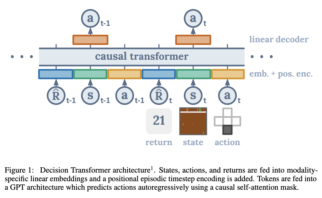
- The Decision Transformers paper showed how RL tasks can be solved with transformer sequence modelling. Figure 1 from their paper describes the critical components of a Decision Transformer.
- A Mathematical Framework for Transformer Circuits that describes how to think about transformers in the context of mechanistic interpretability. Important ideas include the ability to decompose the residual stream into the output of attention heads and MLPs, the QK circuits (decides if to write information to the residual stream), and OV circuits (decides what to write to the residual stream).
- The Understanding RL Vision, which analyses how an RL agent with a large CNN component responds to input features, attributing them as good or bad news in the value function and proposes the Diversity hypothesis - “Interpretable features tend to arise (at a given level of abstraction) if and only if the training distribution is diverse enough (at that level of abstraction).”
Methods
Environment - RL Environments.
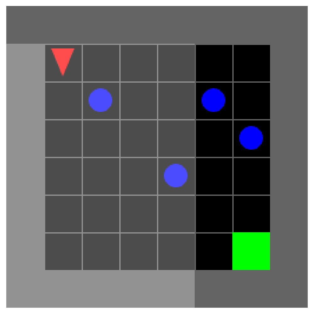
GridWorld Environments are loaded from the Minigrid python package. Such environments have a discrete state space and action space where an embedded agent can turn right or left, move forward, pick up and drop objects such as keys, and use objects such as a key to open a door. Each gridworld involves a different task/environment, and most involve very sparse rewards. The observations can be rendered full or partial (from the agent’s point of view). In this work, we use partial views.
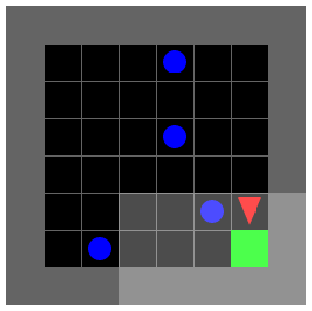
Dynamic Obstacles Environment
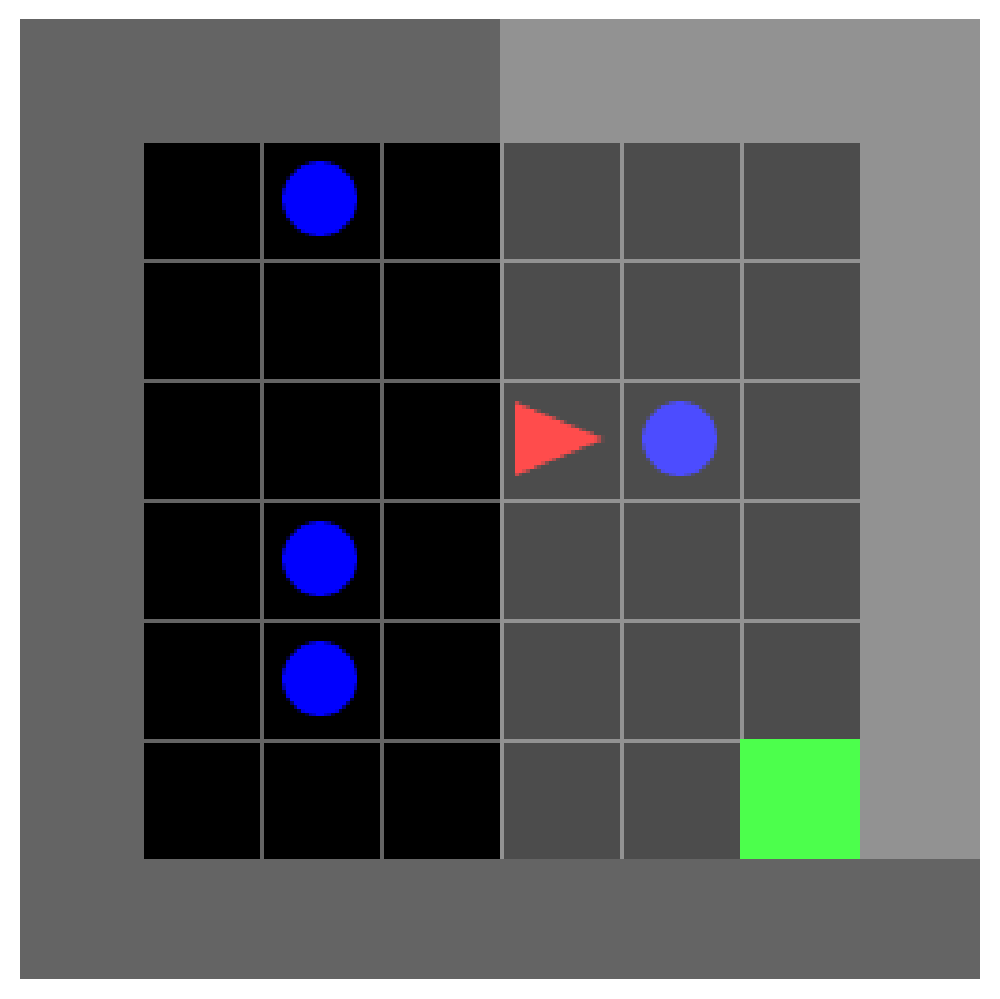
This environment involves no keys or doors. An agent must proceed to a green goal square but will receive a -1 reward if it walks into a wall or obstacle (ending the episode). The obstacles move randomly every timestep, regardless of what the agent does. The agent received 1 reward (or time-discounted reward with PPO). The goal square does not move, and the space is always a fixed-size grid.
Decision Transformer Training
Trajectories are generated with an implementation of the PPO algorithm developed as part of the ARENA Coursework. We modified code from the original decision transformer paper for the model architecture to work with arbitrary mini-grid environments and to use TransformerLens. We flatten observations and use a linear projection to create the state token. We remove tanh activations (used in the original DT architecture in state/RTG/action encodings) and LayerNorm everywhere to have more linearity to facilitate analysis.
Training of the decision transformer is performed as described in the original decision transformer paper, although we have not implemented learning rate schedules.
Attribution and Preference Directions
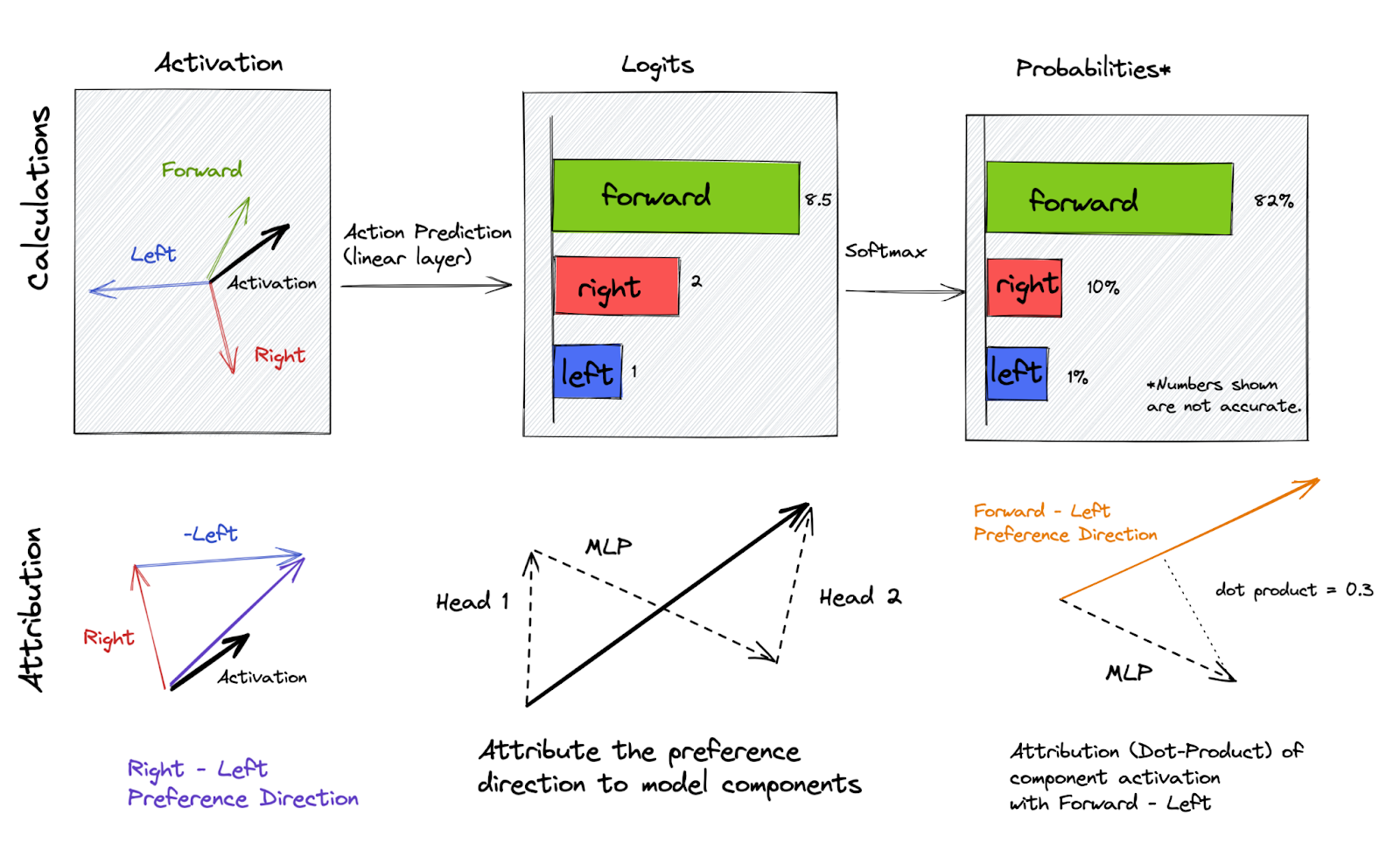
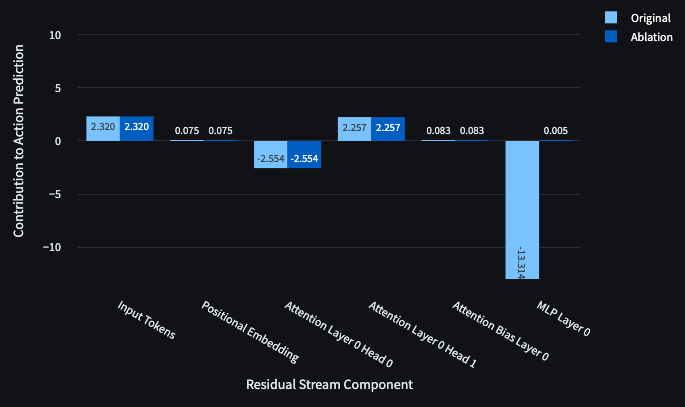
We can perform logit attributions by decomposing the final logits for [forward, left, and right] actions into a sum of contributions for each component (attention heads, MLPs, input tokens). This analysis can be conceived of as a single-step version of the integrated gradients method described in Appendix B of Understanding RL Vision.
However, since softmax is invariant under translation, logits aren't inherently meaningful. It is useful to construct the notion of a “preference direction”, which is the difference between the attribution to one action, such as forward, minus the attribution to another, such as right. Figure 3 shows preference direction decomposition. In the Dynamic Obstacles task studied, the actions possible are only forward/right/left, meaning that the pairwise preference of the model loses some information (an action is left out). Still, we find that right and left logits correlate heavily, making a pairwise analysis useful.
An Interface for live Circuit Analysis
Inspired by OpenAI’s approach to the Interpreting RL Vision project, I built an app in streamlit which would enable me to generate trajectories by playing mini-grid games myself whilst observing analysis of model activations and preferences over actions.
Results
Training a small Decision Transformer
We first trained an RL agent via the proximal policy optimisation (PPO) algorithm, which solved the task well and generated trajectories of varying rewards. Ideally, we might have written specific code to sample PPO agents of varying quality; however, it was much quicker to simply store the trajectories generated during PPO training.
With these trajectories, we trained decision transformers of varying sizes (0, 1, 2 layers) as well as width/hidden dimension size (32, 64, 128), number of heads (2, 4) and context length (1, 3 and 9 timesteps worth of tokens). We evaluated the decision transformer during training by placing it in the dynamic obstacle environment and observing performance when conditioned on high reward.
We found that the transformer that seemed to robustly achieve good performance was a 1 layer transformer with a hidden dimension of 128, two heads and a single time step.
Characterising the calibration of this transformer (to confirm it was a good simulator of trajectories of varying quality and not simply a good agent), we generated calibration curves showing average performance achieved for a range of Reward-to-go’s ( RTGs - the target reward the agent is conditioned to achieve).
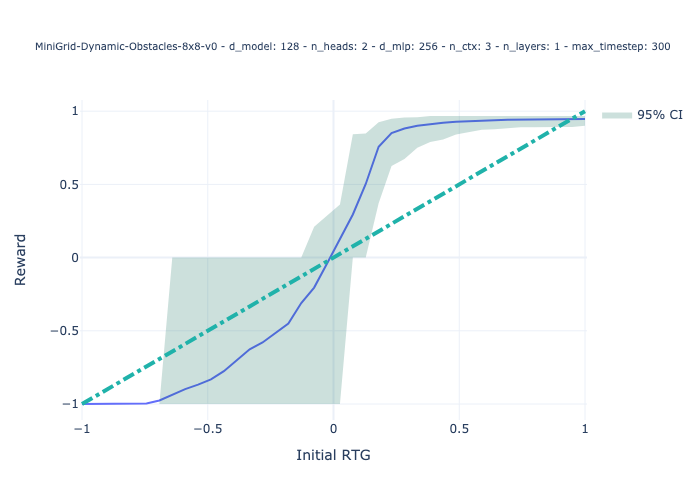
Now Figure 5 appears to show a highly miscalibrated simulator, at least insofar as the curve is s-shaped rather than linear. I would argue, however, that it is certainly good enough for analysis for the following reasons.
- Critical points at RTG = -1, RTG =0 and RTG ~ 1 are unbiased. This means that at -1, the simulated agents are failing pretty robustly; at 0, they are surviving the entire episode (with some variation), and at high RTG, they are succeeding pretty robustly.
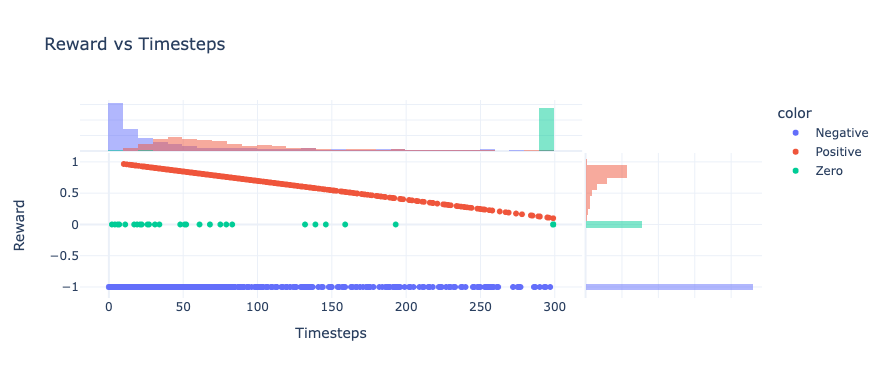
- RTG values between -1 and 0 RTG are never given to the agent in training (Figure 4), so these values shouldn’t really be used to judge the decision transformer.
- To be calibrated for RTG values between 0 (non-inclusive) and 1, the decision transformer must reach the goal in a precise number of steps which is difficult given that obstacles move randomly and can extend the amount of time the agent must take to reach the obstacle. To do this well is likely hard, given that there isn’t much training data for low positive RTG values (Figure 4).
Having trained a decision transformer and verified that it can generate trajectories consistent with various levels of reward, we proceeded to analyse the decision transformer.
Black Box Model Characterisation
To achieve calibrated performance at RTG = -1, RTG =0 and RTG ~ 1, as shown above, the model must robustly learn 3 different behaviours that activate different levels of RTG. Table 3 lists these and their corresponding RTGs. RTG = 1 is impossible to achieve with a time-discounted reward so we use RTG = 0.90 instead.
RTG | -1 | 0 | 0.90 |
Wall Avoidance | yes* | yes | yes |
Obstacle Avoidance | no | yes | yes |
Goal Avoidance | yes | yes | no |
Table 1: RTG Modulated Behaviours. Wall/Obstacle/Goal Avoidance means not walking into those objects. The agent must not reach the goal when RTG is negative nor hit walls or obstacles when it is positive. At 0 RTG, it must avoid walls, obstacles and the goal. *Notably, the agent could learn to achieve -1 RTG by walking into walls but appears not to do so.
Decision Transformer Architecture
The model analysed has a single layer, two attention heads and a context window that only includes the current state and the RTG. Because of the lack of layer norms or non-linearities, which we removed, we can perform an analysis where we decompose the contributions of each component to the preferred direction. Figure 6 describes the architecture.
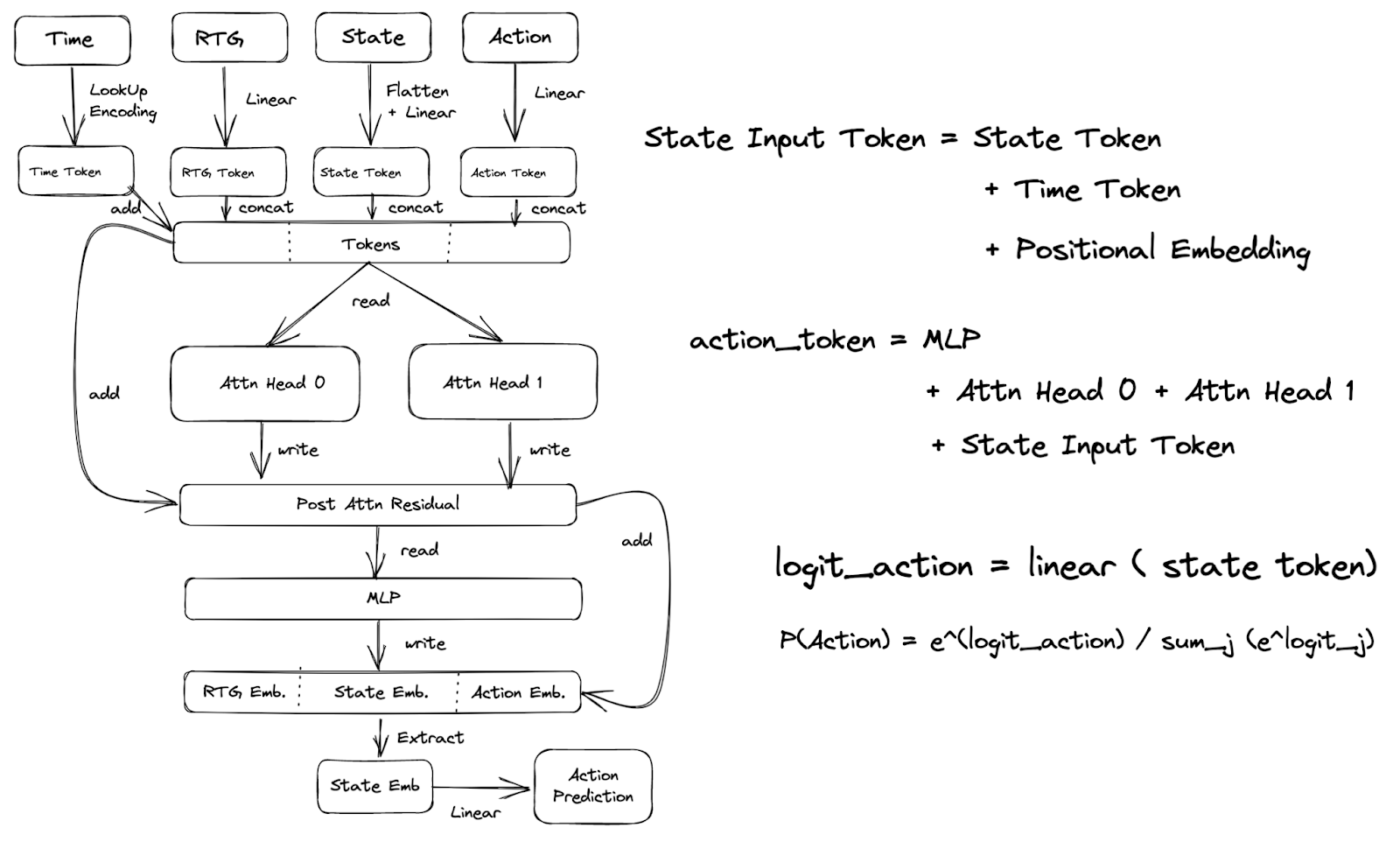
Worth noting:
- Information from the RTG token can be moved to the state embedding (used to predict the action) at the attention heads and not before. So we expect behaviours that are different based on the RTG to occur in those components.
- The state embedding is extracted and used to predict the next action. So the Action embedding is not used in the 1-time step model.
Circuit Results Summary
The analysis in this post involves playing the game, doing ablations, and visualising attributions and weights for different components to try to work out what's happening. I don’t consider any of this rigorous evidence but proof of concept (and practice!).
That being said, the transformer appears to learn various trigrams (RTG, f(State) -> Action) combinations, where f(state) includes things like whether the object in front of the agent is the goal, an obstacle or a wall. There are also broader biases that I haven’t fully understood, such as the tendency to manoeuvre the grid clockwise.
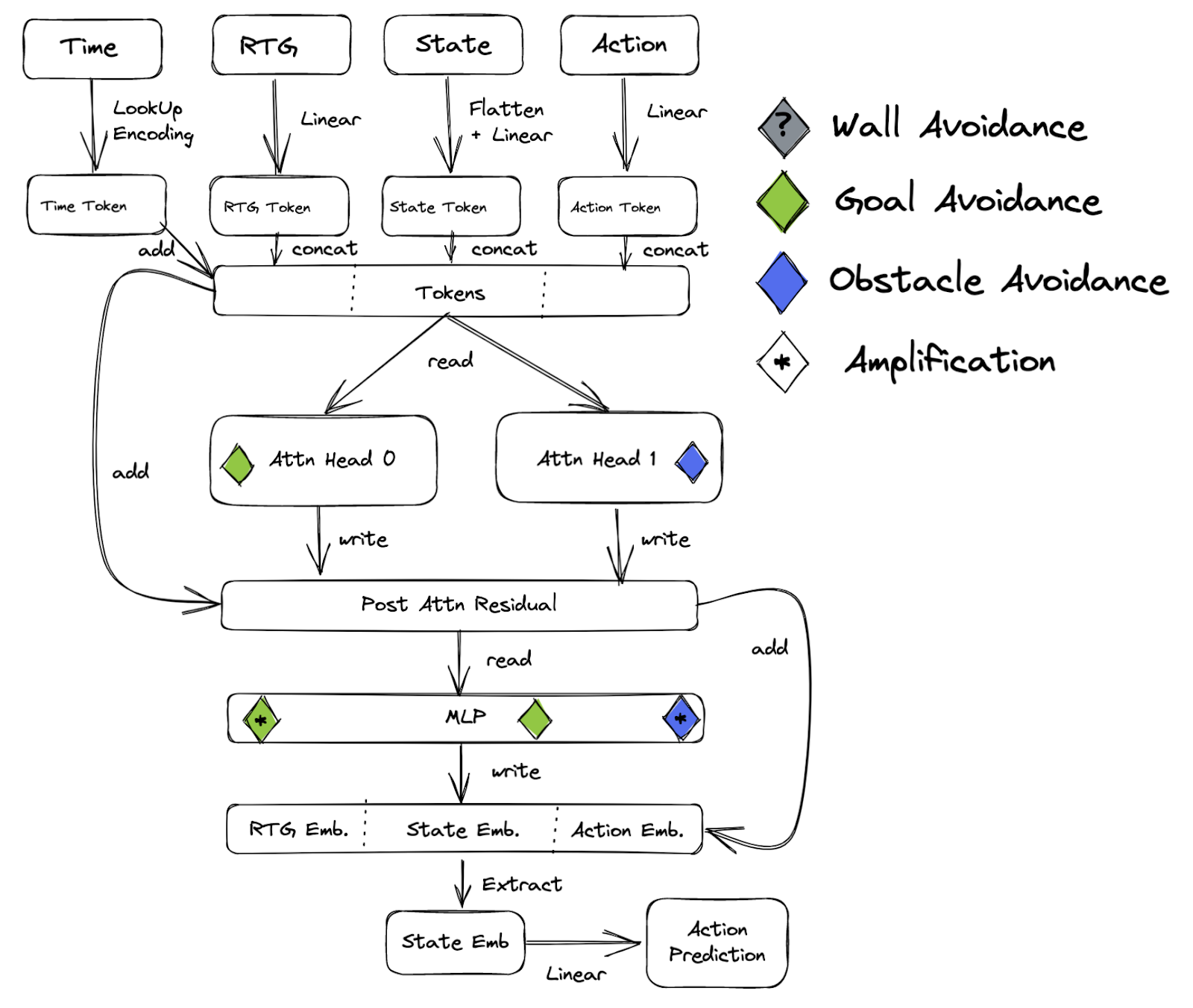
The extent to which these trigrams can be localised to specific components varies, but broadly speaking:
- Head 0 is responsible for goal avoidance at -1 or 0 RTG (from the top) but doesn’t encourage the agent to enter the goal at positive RTG.
- Head 1 is responsible for obstacle avoidance at 0 or positive RTG but doesn’t encourage the agent to walk into obstacles at -1 RTG.
- The MLP amplified head 1 and head 0 contributions and appears responsible for goal avoidance at RTG = -1 (from the left).
The rest of the analysis shows:
- How we localise behaviours via ablations (Head 0 for goal avoidance from the top, Head 1 for obstacle avoidance and MLP for goal avoidance from the left).
- Interpretation of the time/RTG/observation embeddings projecting the forward/right direction in the time and observation embeddings.
- A mechanistic analysis involving the QK and OV circuits of head 1 doing obstacle avoidance.
- The QK circuit attends to the state (not RTG) when there is anything in front of the agent.
- The OV circuit inhibits forward motion when high object channel values are in front of the agent (goals/obstacles).
- Not attending to RTG also inhibits forward motion since RTG projects into forward/right from the residual stream.
If you have no time, skip ahead to the obstacle avoidance circuit. It’s the most interesting section.
Attention and Head Ablation
Inspecting the dot products of components of the residual stream with the forward/right direction can hint at the responsibilities of model components, but performing ablations rapidly demonstrates the value of different components. Looking at each of the behaviours defined above, we ablated Head 0, Head 1 and the MLP one by one and found the following responsibilities, summarised in Figure 7. We used mean ablations for this write-up but found similar results for zero ablation.
To substantiate these results, I’ll share a few example cases. Wall avoidance and Goal seeking are associated with the initial state embedding. This can be seen by inspecting the dot product of this component in the forward/right direction, which is clearly significant when not facing walls (Figure 9) and facing the goal (Figures 8, 10). Wall following in the clockwise directions appears to be contributed to by both heads and the MLP.
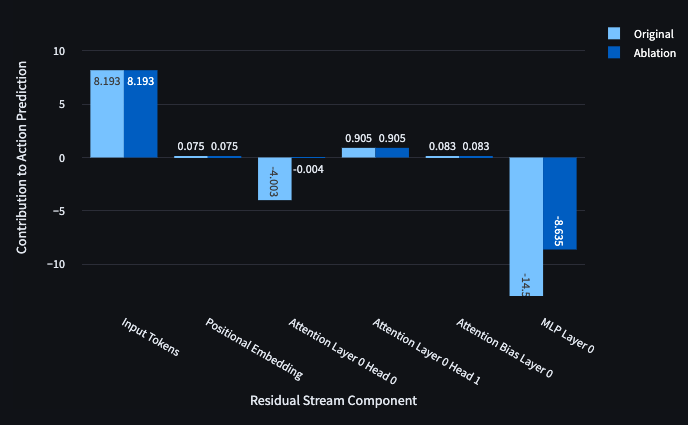
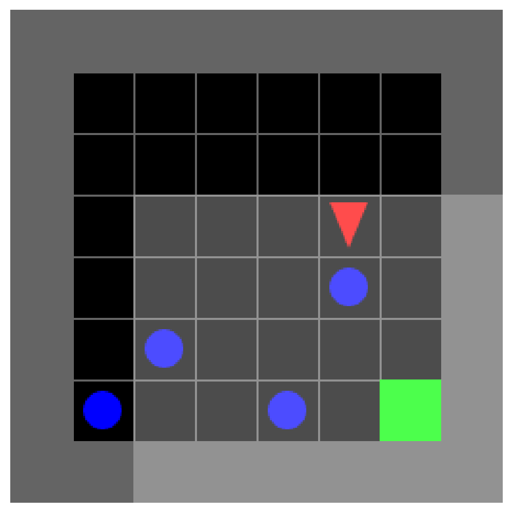
Ablation of Head 0 makes the DT reach the Goal at RTG = -1 from the top
Since an agent which reaches the goal receives a positive reward, the transformer refuses to enter the goal in cases where RTG = -1. However, ablation of Head 0 both directly reduces the projections against the forward/right direction and leads the MLP to contribute less to this negative direction (i.e. right over forward).
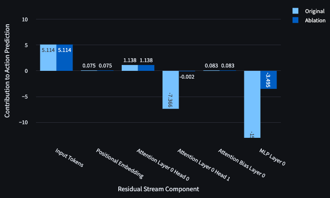
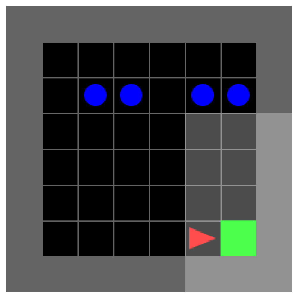
Ablation of Head 1 makes the DT hit obstacles at RTG = 0.9
Since an agent which walks into an obstacle receives a negative reward, the transformer refuses to walk into obstacles to the goal in cases where RTG is > 0.2-0.3. However, the Ablation of Head 1 directly reduces the projection against the forward/right direction and leads the MLP to contribute less to the opposing direction.
Ablation of MLP makes the DT approach the Goal at RTG = -1 from the left
Since an agent which reaches the goal receives a positive reward, the transformer refuses to enter the goal in cases where RTG = -1. We’ve seen that ablating head 0 can encourage entering the goal from the top. However, it appears that Head 0 does not likewise inhibit forward into the goal from the left. In fact, ablation of the MLP will do this.
Analysing Embeddings
Having found concrete evidence showing us where various behaviours originate in our model, we can start going through the model architecture to see how the model reasons about each of the inputs.
Analysing the RTG and Time Tokens
Reward-to-Go
The Reward-to-Go token is a linear projection of one number, the RTG. For the RTG to affect the decision of the transformer, the “information” in this token must be moved to the state token, which will be projected onto the action prediction.
Nevertheless, it appears the network learnt to project almost 1:1 in the forward/right direction as the dot product of the RTG embedding with the forward/right direction is ~1.13 (This means if the information was moved to the state token it would contribute to forward/right). The dot product of the right/left direction with the RTG embedding is ~ -0.16. This can be interpreted as the RTG embedding encouraging forward movement and probably being fairly ambivalent with rest to right/left when this embedding is attended to in the attention heads later in the model.
Time
The Time embedding is a learned embedding that essentially functions as a learned look-up table of vectors as a function of the integer time value. Unlike a positional embedding in a regular transformer, which is of the same form, this embedding is added to groups of 3 tokens which make up one timestep, an RTG, a state, and an action group. The time embedding is added to the state token (and RTG token).
Analysing the State Embeddings
Minigrid uses a 3-channel encoding scheme, providing the agent with information about the objects, colours and states in a 7 by 7 grid around itself (when you use a partial observation view, which we do in this project). Figure 12 is useful for understanding the Minigrid observation encoding schema
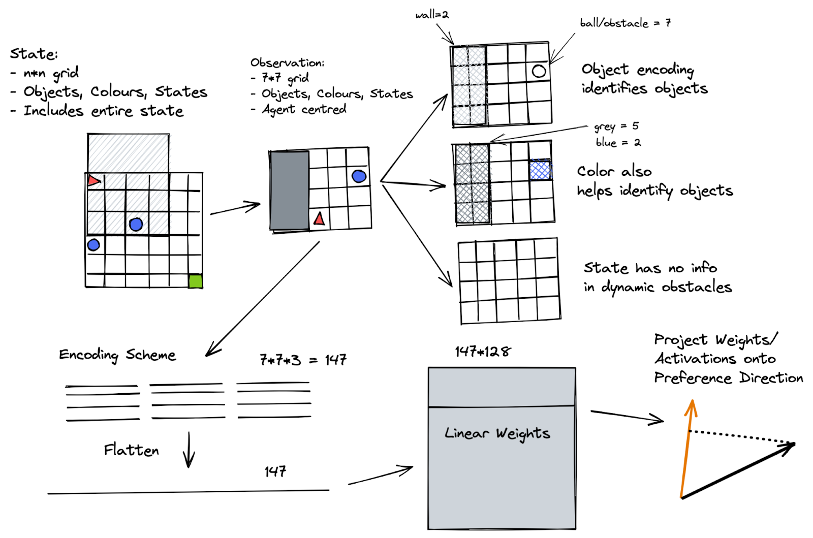
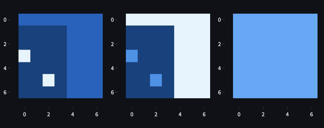
Since I hadn’t thought about it until a decent way through my original analysis, I didn’t one-hot encode the state. This introduces a significant inductive bias induced by spurious index ordinality. For example, in the object channel, the goal is 8, and the obstacle (ball) is 6. So an obstacle looks like ¾ s of the goal, which is really dumb.
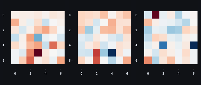
Figure 13 visualises each channel of the state/observation, with colour representing the index. In the object view, obstacles are more distinguishable from empty space than in the colour channel. The state channel provides no information since it’s used to show whether doors/boxes are locked, unlocked or open, which isn’t relevant to the Dynamic Obstacles task.
This inductive bias led to a weird behaviour where agents would successfully avoid the obstacles but also try to avoid the goal square. This was fixed when I started over-sampling the final step of trajectories, a hack I think wouldn’t be necessary for the one-hot encoded version of the model but is also a generally good trick for getting agents to train faster on mini-grid tasks.
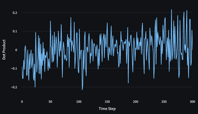
It’s possible to look at the activation at each position in each channel projected into the forward/right direction since each position in each channel projects into the residual stream (128 dimensions) which is itself eventually projected into the action logits (see Figure 14).
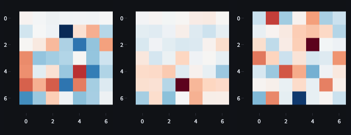
There are a few interpretations worth taking away from here:
- this may look fairly noisy because these neurons are doing lots of other things whilst also projecting directly onto the preference direction.
- It’s also possible that collectively they project onto the preference direction quite cohesively, but there are strong correlations between features leading to hard-to-interpret or dispersed processing (diversity hypothesis type problem).
Nevertheless, I do think there is some valuable information in Figure 14. We know from our observations above that the state embedding mostly works as a wall detector.
The square in front of the agent in the colour embedding has a large negative value (-0.742). Empty Squares are 0 in colour, obstacles are 2, and walls are 5. This square thus will project weakly onto “don’t walk forward when there is an obstacle in front” and strongly onto “don’t walk forward when there is a wall in front”.
The square in front of the agent in the object embedding (left in Figure 14) has a slightly positive value (0.27), so it encourages walking into walls and obstacles but encourages walking into the goal square more than other objects.
This is cool because it suggests that the inductive bias associated with my idiotically not one-hot-encoding the vision is directly why the model avoids walls much more strongly than it avoids obstacles. It also explains why early versions of the model avoided the goal square.
I’ll make a table to show how the two neurons for object/state embedding for the square directly in front of the agent combine to respond to objects/colours.
Object/ Colour | Object Value | Colour Value | Positional Contribution to Forward/Right |
| Empty Space | 1 | 0 | 0.27 * 1 = 0.27 |
| Wall | 2 | 5 | 0.27 * 2 - 5 * 0.742 = -3.17 |
| Obstacle | 6 | 2 | 0.27 * 6 - 2 * 0.742 = 0.136 |
| Goal Square | 8 | 1 | 0.27 * 8- 1 * 0.742 = 1.42 |
Table 3: Back of Envelope Calculation for Object and Colour Embeddings activations dot product with forward/right direction for the position directly in front of the agent. The results suggest embedding functions as a strong wall avoider and a weak goal square seeker.
Table 3 provides evidence for how the state embedding detects walls directly in front of the agent. However, there are lots of other neurons projecting into the forward/right direction in the state embedding, as shown in Figure 15.
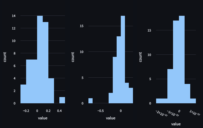
Let’s summarise:
- You might have expected that the state embedding wouldn’t project directly in any preference directions. In practice, sometimes we see it does, suggesting that besides likely encoding features, it is directly informing the model's output (which we saw in the residual stream dot product contributions earlier).
- Using attribution, we can see that the model uses a combination of colour and object channels to detect walls directly in front of the agent and use this to inhibit forward motion.
- Analysis of the state encoded positions does not suggest information is only being read from the square in front of the agent, but rather many parts of the view, suggesting the decision transformer may be using other information such as possibly regions walls vs empty space.
Explaining Obstacle Avoidance at positive RTG using QK and OV circuits
To explain how our decision transformer avoids obstacles at positive RTG, we can reference the QK and OV circuits, the encoding scheme, and the RTG attribution. Briefly, the QK (Query-Key) circuit controls which token the head attends to, and the OV (Output-Value) circuit determines how attending to each token affects the logits. More details are here.
First, we need the circuit to activate at a higher RTG. The circuit needs to inhibit moving forward (which we’ll approximate roughly with the forward/right direction), so it will want to attend to the state (not the RTG, since we know it will project positively into forward/right direction and the forward logit).
Attention to the RTG will be high where the query and key vectors match (key/source is the RTG token and the query/destination token is the state). The QK circuit visualisation in Figure 16 shows how values RTG attention is inhibited by anything that isn’t an empty square in front of the agent.
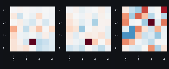
Now, we can look at the OV circuit for attention head 1 to determine the effect on the output from attending to the state rather than the RTG (Figure 17). It appears that high object channel values in front of the agent will lead to a decrease in the forward logit. This includes obstacles (6) and the goal (8) (see table 3).
Lastly, it’s worth noting that the MLP tends to accentuate the output of either attention head, helping them project strongly enough to counteract the strong forward/right projection we usually see coming from the state embedding when not facing a wall. Thanks to Callum for pointing out that we can measure cosine similarity between input directions of MLP neurons and directions of the OV circuit to provide more detail here. I plan to do this soon.
Discussion
Analysis takeaways
- Details of the Decision Transformer
- The Decision Transformer learns several robustly true relationships in the trajectories and reflects these relationships with its own behaviour.
- These behaviours can be localised to specific components, such as the two attention heads.
- Embeddings in this decision transformer were highly interpretable because they had a high product with preference directions.
- QK (state to RTG) and OV (action from the state) circuits are highly interpretable.
- Inductive Biases and Encoding Schemas matter.
- The feature use/algorithms implemented by the decision transformer were highly dependent on the encoding scheme, which provided strong and counter-intuitive inductive biases, such as in table 3, where we see linear combinations of channel/colour encodings used to make the state encoding promote wall avoidance, goal entrance but be ambivalent to obstacles/balls.
- The diversity hypothesis felt like a helpful framing
- Plenty of signals in this experiment (the state space mainly) have spurious correlations. The walls are next to each other, and the goal square is always in the corner. Even the colour of the goal square is always the same. This gives the models many ways to read environmental features beyond the obvious ones. When the model does this, it’s much harder to work out why it’s doing what it is doing. I’m still unclear about some of this model's details, partly because of this.
- It is possible to thoroughly understand a decision transformer by cooperative play with concurrent analysis.
- Ablation was wildly useful for localising behaviours/contextual responses (suggesting activation patching might also be useful, even though it might have been overkill for this model).
- Watching the dot products of embeddings/component output in the forward/right direction was also helpful for finding relevant components.
Limitations
Some limitations worth highlighting:
- The mechanistic interpretability methods used here operate on a tiny, simple decision transformer. They rely on linearity between the transformer output and the logits over decisions. The model used doesn’t have layer norms and uses a tiny context window (so there’s none of the same complexity that might exist in a model with attention across a larger context window), has only 1 layer, and an output vocabulary of 3 actions. As such, the fact that interpretability works in this context is only weak evidence that interpretability will be possible in more complicated decision transformers.
- My analysis has not been super rigorous. I opted to create an interactive environment with high visibility into the agent's decision-making and used linear attribution analysis only. This has some advantages but means that if counter-examples existed, they might not be pronounced. I hope to mitigate this risk by sharing the interactive app and encouraging others to explain their observations about the model, but by developing more comprehensive methods in the future.
I tweaked hyperparameters to encourage as interpretable a model as possible. This means training for a long time with no meaningful loss decrease to encourage weight decay to favour a generalising solution over a memorising solution [LW(p) · GW(p)]. I suspect that, in many cases, models can be performant and lack nice abstractions.
Alignment Relevance
A more general list of why MI might be useful to AI alignment is provided here [LW · GW].I think that Decision Transformer MI might be useful to AI alignment in several ways:
- Retargeting the Search [LW · GW]. The ELI5 on this post is “understand how the AI works out what it wants and make it want what you want”. John Wentworth’s post makes a case for this approach being a “true reduction of the problem”, and creating an empirical research area around retargeting the search (and understanding the AI’s internal concepts/reasoning) seems like a robustly good thing to do. Decision Transformers enable us to do this in a much simpler context than large language models, but in which the notion of goals and an AI’s internal language feels somewhat natural. I picked the simplest possible problem I thought would work for this. The results make me optimistic about moving to tasks where we might find something akin to search (like maze solving, for example) or other tasks with instrumental goals.
- Providing Mechanistic Explanations behind Goal Misgeneralization/Reward Mis-specification. Goal misgeneralization has been studied in simple RL tasks where we might plausibly be able to train decision transformers and interpret them. If circuit universality holds, then insights from decision transformers might transfer to other architectures. Still, even if they don’t, most LLMs are transformers, so I’d expect insights to be useful anyway.
- (The instrumental goal of) Giving Mechanistic Interpretability a middle ground. MI is a growing field with lots of low-hanging fruit (like this project!). Decision Transformers give circuits and features a slightly different flavour. RTG modulation (see the RTG scan analysis) seems like it could be potent as a way to help us find circuits. Being able to vary RTG and thus behaviour feels like flashing lights on and off from a distance to draw attention to them. This work showed that at least basic interpretability is possible in this context, which gives us an intermediate between algorithmic tasks and LLM. Decision Transformers also obviously bring interpretability into the context of many RL tasks and have elements of multi-modality (tokens can represent visual input, the specified reward, and previous actions), and states can have text components such as in some mini-grid tasks and in GATO.
Capabilities Externalities Assessment
I believe strongly that given the precipice we find ourselves standing on, it behoves everyone publishing empirical work to consider how it might backfire from an alignment perspective. Part of this means making a public commitment to care about capabilities, which you can consider as doing. I promise you, seriously if you think this or any other work I’m doing might enhance capabilities. If you feel this is the case, please consider the best way to notify me of this, probably an email (so as not to highlight any capabilities enhancing insight further in a public forum) but feel free to CC anyone you think would be a reasonable third party.
Before publishing this work, I considered several factors and spoke to various alignment researchers. I have published it because it is a reasonable trade-off between empirical progress on alignment and possible capabilities enhancement.
For reference, here are some posts on capabilities/MI.
- The Defender’s Advantage of Interpretability - LessWrong [LW · GW]
- Chris Olah’s views on AGI safety - LessWrong [LW · GW]
Future Directions
This project was designed to provide early feedback for what could be a much longer research investigation involving larger systems and more comprehensive analyses followed by interventions such as model editing.
- Mainline experiment extensions:
- Implement extra analyses such as activation patching or checking for composition directly between attention heads and MLPs.
- Start working on larger/harder RL tasks that involve more complicated algorithms and/or search and/or alignment relevant phenomena such as goal misgeneralization. The way I see this going is Minigrid D4RL < ProcGen < Atari < whatever tasks Gato does.
- I’m probably going to design environments/tasks to force the model to learn all the best abstractions, like moving the goal square around, and changing the colour of the obstacles and the goals (or don’t bother passing through colour). This might help us work out how crisp the model's abstractions need to be for different techniques to detect them and extend our interpretability techniques to many models despite the diversity hypothesis.
- Key challenges will involve:
- Finding/generating training data for all the tasks we want to learn:
- Perfecting/improving trajectory collection (currently, I use whatever was generated by the PPO agent during training, but learning a simulator is harder than learning a single agent, so it’s possible we’ll want more/better-sampled data).
- Adapting the analysis code to facilitate these other environments.
- The input visualisation code will need to change a lot.
- Once the context window is larger and there are more layers, finding circuits will be more involved. Writing the analysis code to find head composition, working out how to circuit analysis in decision transformers, and other tasks all seem non-trivial.
- Finding/generating training data for all the tasks we want to learn:
- Auditing [LW · GW] Games [LW · GW]/High-level Interpretability:
- It could be interesting to start training many different decision transformers on a variety of tasks and use them for auditing games (an adversarial framework for testing our interpretability methods).
- Model Editing
- As we understand DT agents performing these tasks, model editing techniques could fix things like goal misgeneralisation or improve RTG calibration curves.
- Moreover, I’ve been thinking about how we might be able to practise retargeting the search and think manually editing decision transformers in non-trivial ways would be a cool proof of concept.
- Mechanistic Anomaly Detection [LW · GW]
- Precisely because none of the methods used in this project would have detected weird edge cases in model behaviour, I think it is interesting to think about how not only current MI tools could be used to better explain the model's behaviour, but how we might specifically design MAD type algorithms in the context of decision transformers.
- Possibly, it’s worth taking inspiration from Understanding RL Vision and finding “hallucinations” in the visual/state processing. Can we mechanistically distinguish between hallucination/adversarial inputs and genuine observation processing at runtime? (i.e., investigate the activation cache or a small subsection and flag a decision as anomalous prior to letting the agent execute it).
- The Diversity Hypothesis and Grokking
- Understanding RL Vision suggests that further research could attempt to validate the diversity hypothesis (I think this would be a good domain to attempt that, at least as one piece of the puzzle).
- Furthermore, since Neel has built some intuitions [LW(p) · GW(p)] about generalisation in the context of transformers, some work might be done that intersects both grokking/RL and could speak to the diversity hypothesis.
- (I found some evidence that my model was performant long before it was interpretable, but training loss had hit a plateau, and I am interested in creating model checkpoints and being more thorough about what I saw).
- A new domain for Mechanistic Interpretability
- Last, but not least, all the usual demons still exist and will probably present many challenges.
- What do circuits look like in Multi-Modal models? How will information like “the key is already picked up” or “I should be looking for a blue door, not a green door” get stored?
- Superposition might take on a different flavour in these tasks since there might be unusual joint distributions of feature occurrence causing unusual interference patterns.
- Finding ways to automate circuit analysis/interpretability could be good too. Maybe something like a wrapper around the agent/cache which takes a snapshot of every time qualitatively different mechanisms appear and creates a bank of “scenarios” for analysis. In this case, it would have been something like all the different scenarios for something in front of the agent, the scenarios of walls/corners on different sides of the agent etc.
Meta
Acknowledgements
I’m very grateful to
- Paul for suggesting the idea for this project and for all the great collaboration!
- Callum McDougall and Matt Putz for running the ARENA program, the other ARENA participants and SERI MATS scholars for all their chats with me about this, and Conjecture for hosting ARENA.
- Jacob Hilton for writing up his curriculum, which formed the basis of ARENA and for his weekly calls with the ARENA Participants.
- Neel Nanda for endorsing an early description of this project which was a significant factor in my choosing to start it. Also, I’ve been using your post as a rough guide for structuring this post, so thanks for that.
- Also, this work would not have been possible without TransformerLens, so double-thanks to Neel.
- My regrantor. Thank you so much!
- Ruby, who gives better advice than I ever realise I’m getting at the time.
Many thanks to all the people who have given feedback on this draft, including Callum McDougal, Dan Braun, Jacob Hilton, Tom Lieberum, Shmuli Bloom and Arun Jose.
Author Contributions
Paul Colognese wrote up the initial project description, and he, Joseph and Callum McDougall had a few early meetings to discuss the project. The PPO algorithm was almost entirely taken from the ARENA curriculum written by Callum, based on MLAB content. The Decision Transformer code was based heavily on the original code base, which is still a submodule of the GitHub repository.
The rest of the work, building the code base, training the agents, building the interactive app and writing this post, was done by Joseph Bloom, whose perspective the write-up is written in.
Feedback
Please feel free to provide feedback below or email me at jbloomaus@gmail.com. The GitHub repository is a reasonable place for technical feedback. Feedback on the app/codebase would be appreciated too!
Glossary
I highly recommend Neel’s glossary [LW · GW] on Mechanistic Interpretability.
- DT/Decision Transformer. A transformer architecture applied to sequence modelling of RL tasks to produce agents that perform as well as the RTG suggests they should.
- State/Observation: Generally speaking, the state represents all properties of the environment, regardless of what’s visible to the agent. However, the term is often used instead of observation, such as in the decision transformer paper. To be consistent with that paper, I use “state” to refer to observations. Furthermore, mini-grid documentation distinguishes “partial observation” which I think of when you say observation. Apologies for any confusion!
- RTG: Reward-to-Go. Refers to the remaining reward in a trajectory. Labelled in training data after a trajectory has been recorded. Uses to teach Decision Transformer to act in a way that will gain a certain reward in the future.
- Token: A vector representation provided to a neural network of concepts such as “blue” or “goal”.
- Embedding: An internal representation of a token inside a neural network.
- Full QK Circuit: The calculation of the attention patterns is determined by the full QK circuit. This determines how information is moved between tokens in attention heads.
- Full OV Circuit: The calculation of the attention head output only depends on the value and output weight matrices (and embedding/unembedding matrices).
- The diversity hypothesis: “Interpretable features tend to arise (at a given level of abstraction) if and only if the training distribution is diverse enough (at that level of abstraction).”
- Attribution: A measurement indicating the relationship between activations of neurons/layers in a neural network at one stage and another. Action attribution is a measurement of activation at one or more layers contributing to the final action logit magnitudes.
- Preference Direction: The difference between the attribution to one action, such as forward, minus the attribution to another of a vector in the residual stream. Used to indicate how components added to the residual stream of the transformer affect its action preferences.
13 comments
Comments sorted by top scores.
comment by Oskar Hollinsworth (oskar-hollinsworth) · 2023-03-08T14:23:25.436Z · LW(p) · GW(p)
Really interesting and impressive work, Joseph.
Here are a few possibly dumb questions which spring to mind:
- What is the distribution of RTG in the dataset taken from the PPO agent? Presumably it is quite biased towards positive reward? Does this help to explain the state embedding having a left/right preference?
- Is a good approximation of the RTG=-1 model just the RTG=1 model with a linear left bias?
- Does the state tokenizer allow the DT to see that similar positions are close to each other in state space even after you flatten? If not, might this be introducing some weird effects?
↑ comment by Joseph Bloom (Jbloom) · 2023-04-17T12:37:17.825Z · LW(p) · GW(p)
My apologies! I thought I had responded to this. Better late than never. All reasonable questions.
"What is the distribution of RTG in the dataset taken from the PPO agent? Presumably it is quite biased towards positive reward? Does this help to explain the state embedding having a left/right preference?"
The RTG distribution taken from the PPO agent is shown in Figure 4. It is the marginal distribution of reward, since the reward only occurs at the end of the episode, the RTG and Reward distributions are identical more/less.
If you are referring to the tendency for the agent conditioned on low RTG (0.3) to get RTG closer to (0.8) as "biased towards positive reward". I think this is a function of the training distribution which includes way more RTG~0.8 than 0.3 so yes.
The state embedding having a left/right preference is probably a function of the PPO agent getting success going clockwise, this being reinforced and then this dominating the training data for the DT.
"Is a good approximation of the RTG=-1 model just the RTG=1 model with a linear left bias?"
I'm not sure what you mean by "linear left bias". the RTG=-1 model behaves characteristically differently (see table 1).
"Does the state tokenizer allow the DT to see that similar positions are close to each other in state space even after you flatten? If not, might this be introducing some weird effects?"
Yes I believe the encoding used had that property. I've seen replicated these results with a less nasty encoding and the results are mostly similar if a little easier to interpret.
comment by TurnTrout · 2023-02-07T18:15:35.774Z · LW(p) · GW(p)
The ablations seems surprisingly clear-cut. I consider myself to be very on board with "RL-trained behaviors are contextually activated and modulated", but even I wasn't expecting such strong localization.
To be calibrated for RTG values between 0 (non-inclusive) and 1, the decision transformer must reach the goal in a precise number of steps which is difficult given that obstacles move randomly and can extend the amount of time the agent must take to reach the obstacle. To do this well is likely hard, given that there isn’t much training data for low positive RTG values (Figure 4).
Seems to me that randomness wouldn't prevent the agent from bieng calibrated, because even though any given episode might deviate from the prescribed number of steps, on average the randomness can (presumably) be made to add up to that number. EG it might be hard to bump into the goal after exactly 14 steps due to random obstacles, but I'd imagine ensuring this falls between 10 and 18 steps is feasible?
This inductive bias led to a weird behaviour where agents would successfully avoid the obstacles but also try to avoid the goal square.
This seems like an important manifestation of "models don't 'get reward' [LW · GW], they are shaped by reward [LW · GW]"; even on a simple task where presumably agents can fully explore all relevant options. The e.g. observation encoding (where an obstacle is "3/4" of a goal) matters when predicting what behavioral shards & subroutines get trained into the policy, or considering what e.g. early-stage policies will be like.
(I thiiink I weakly predicted this particular behavior in advance, when I read about the encoding.)
You might have expected that the state embedding wouldn’t project directly in any preference directions. In practice, sometimes we see it does, suggesting that besides likely encoding features, it is directly informing the model's output (which we saw in the residual stream dot product contributions earlier).
Wait, how? Isn't the state observation constant in this task? I'm guessing you're discussing something else?
Replies from: Jbloom↑ comment by Joseph Bloom (Jbloom) · 2023-02-07T21:41:34.019Z · LW(p) · GW(p)
The ablations seems surprisingly clear-cut. I consider myself to be very on board with "RL-trained behaviors are contextually activated and modulated", but even I wasn't expecting such strong localization.
Neither was I. After the fact, it seems easy to come up with reasons why this might be the case. I think measuring this with something like excluded loss might enable a more precise quantification of exactly how localised it was. I also don't see strong reasons to expect this to generalise to larger models. If I see similar results when the task is more complicated, the model is bigger and especially with a larger context window, then I will be more interested in trying to precisely describe how/why/when you get more localisation.
Seems to me that randomness wouldn't prevent the agent from bieng calibrated, because even though any given episode might deviate from the prescribed number of steps, on average the randomness can (presumably) be made to add up to that number. EG it might be hard to bump into the goal after exactly 14 steps due to random obstacles, but I'd imagine ensuring this falls between 10 and 18 steps is feasible?
I think you might be right in the infinite training data regime, where I would expect it to be unbiased however I suspect that the training data being sparse, especially in the low positive RTG reason is enough to make the signal weak. The loss incurred by finishing in the wrong number of steps is likely very small compared to failing when you have positive RTG or succeeding when you have positive RTG, so it could also be that the model doesn't allocate much capacity to being well-calibrated in this sense.
This seems like an important manifestation of "models don't 'get reward' [LW · GW], they are shaped by reward [LW · GW]"; even on a simple task where presumably agents can fully explore all relevant options. The e.g. observation encoding (where an obstacle is "3/4" of a goal) matters when predicting what behavioral shards & subroutines get trained into the policy, or considering what e.g. early-stage policies will be like.
I thought this too and should have remembered to cite "Reward is not the Optimization target". I feel like that concept is now more visceral for me. A relevant takeaway that may or may not be obvious is that simulators with inductive biases might be better/worse at simulating particular stuff as a function of their inductive biases. In this case, the positive RTG range was more miscalibrated as a result of the bias.
Wait, how? Isn't the state observation constant in this task? I'm guessing you're discussing something else?
I'm not sure what you mean by constant. If it were constant then the agent/obstacles wouldn't be moving? I'll elaborate a little bit in case that helps.
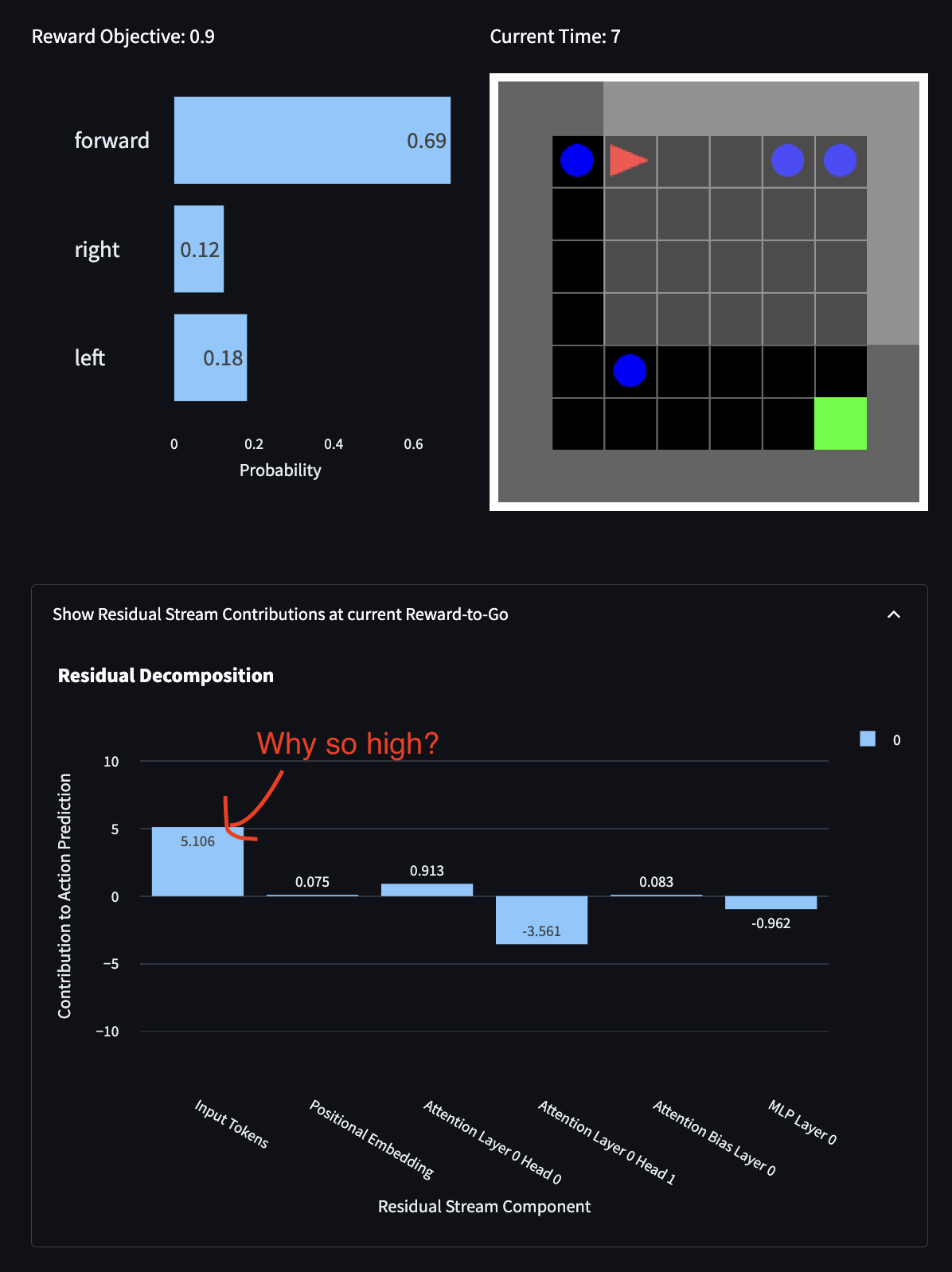
Since RTG gives information about whether the agent should go forward/not in many contexts, you might have expected (although now I think I wouldn't) the residual stream embedding for the state token not to directly contribute to one logit over another before RTG has been seen. In practice, it seems like it does. For example, in this situation (picture below from the app) with RTG = 90, there is a wall to the left of the agent and the state appears to strongly encourage forward/right. I interpret this as as "some agent behaviours are independent of RTG and can be encouraged as a function of the observation/state before RTG is seen".
To clear up some language as well:
- state encoding -> how is the state represented? weird minigrid schema.
- state token -> the value of a state represented as a vector input to the model.
- state embedding -> an internal representation of the state at some point in the model.
I should have written state-token not state-embedding in the quotes paragraph. Apologies if this led to confusion.
comment by TurnTrout · 2023-02-07T17:37:15.666Z · LW(p) · GW(p)
This looks cool, going to read in detail later.
Start working on larger/harder RL tasks that involve more complicated algorithms and/or search and/or alignment relevant phenomena such as goal misgeneralization. The way I see this going is Minigrid D4RL < ProcGen < Atari < whatever tasks Gato does.
Note that team shard (MATS stream) is already doing MI on procgen. I've been supervising/working with them on procgen for the last few weeks. We have a nice set of visualization techniques, have reproduced some of Langosco et al.'s cheese-maze policies, and overall it's been going quite well.
Replies from: Jbloom, None↑ comment by Joseph Bloom (Jbloom) · 2023-02-07T21:07:51.728Z · LW(p) · GW(p)
Thank you for letting me know about your work on procgen with MI. It sounds like you're making progress, particularly I'd be interested in your visualisation techniques (how do they compare to what was done in Understanding RL Vision?) and the reproduction of the cheese-maze policies (is this tricky? Do you think a DT could be well-calibrated on this problem?).
Some questions that might be useful to discuss more:
- What are the pros/cons of doing DT vs actor-critic MI? (You're using Actor-Critic of some form?). It could also be interesting to study analogous circuits in the DT vs AC scenarios.
- I haven't done anything with CNNs yet, for simplicity, but I might be able to calibrate my expectations on the value/challenges involved by chatting to the team shard MATS stream.
Glad to hear your progress is going well! I'll be in the Bay Area for EAG if anyone from the team would like to chat.
Replies from: TurnTrout↑ comment by TurnTrout · 2023-02-14T00:14:17.912Z · LW(p) · GW(p)
We're studying a net with the structure I commented below [LW · GW], trained via PPO. I'd be happy to discuss more at EAG.
Not posting much publicly right now so that we can a: work on the research sprint and b: let people preregister credences in various mechint / generalization propositions, so that they can calibrate / see how their opinions evolve over time.
↑ comment by [deleted] · 2023-02-08T01:00:17.539Z · LW(p) · GW(p)
Are you using decision transformers or other RL agents on procgens ? Also, do you plan to work on coinrun ?
Replies from: TurnTrout, Jbloom↑ comment by TurnTrout · 2023-02-13T23:39:39.911Z · LW(p) · GW(p)
We're analyzing the mech-int-ungodly Impala architecture, from the paper. Basically
=== Impala
conv
maxpool2D
---- residual x2:
relu
conv
relu
conv
residual add from input to this residual block
=== /IMPALA
(repeat 2 more impalas)
---
relu
flatten
fully connected
relu
---
linear policy and value heads
so this mess has sixteen conv layers, was trained on pixels. We're not doing coinrun for this MATS sprint, although a good amount of tooling should cross over.
This has presented some challenges -- no linearity from decomposing an ongoing residual stream into head-contributions.
↑ comment by Joseph Bloom (Jbloom) · 2023-02-08T01:36:05.434Z · LW(p) · GW(p)
comment by Victor Levoso · 2023-02-08T01:47:18.922Z · LW(p) · GW(p)
Oh nice, I was interested on doing mechanistic interpretability on decision transformers myself and had gotten started during SERI MATS but now was more interested in looking into algorithm distillation and the decision transformers stuff fell to the wayside(plus I haven't been very productive during the last few weeks unfortunately). It's too late to read the post in detail today but will probably read it in detail and look at the repo tomorrow. I'm interested in helping with this and I'm likely going to be working on some related research in the near future anyway. Also btw I think that once someone gets to the point that we understand what's going on the setup from the original dt paper it would be interesting to look into this: https://arxiv.org/abs/2201.12122
Also the dt paper finds their model generalizes to bigger rtg than the training set in the seaquest env and it would be interesting to get a mechanistic explanation of why that happens (tough that's an atari task and I think you are right in that that's probably going to have to come later cause CNN are probably harder to work with).
Another thing to note is that OpenAI's VPT while it's technically not a decision transformer (because it doesn't predict rewards if I remember correctly) it a similar kind of thing in that is Ofline RL as sequence prediction, and is probably one of the biggest publicly avaliable pretrained models of this kind. There's also multiple open source implementation of Gato that could probably be interesting to try to do interpretability on. https://github.com/Shanghai-Digital-Brain-Laboratory/BDM-DB1
Also training decision transformers on minerl(or in eleuther's future minetest enviroment) seems like what might come next after atari(the task gato is trained are mostly atari games and google stuff that is not publicly avaliable if I remember correctly)
(sorry if this is too rambly I'm half asleep and got excited because I think work on dt is a very potentially promising area on alignment and was procrastinating on writing a post trying to convince more people to work on it, and I'm pleasantly suprised other people had the same idea)
Replies from: Jbloom↑ comment by Joseph Bloom (Jbloom) · 2023-02-08T06:07:27.146Z · LW(p) · GW(p)
Hi Victor,
Glad you are keen on this area, I'd be very happy to collaborate. I'll respond to your comments here but am happy to talk more after you've read the post.
The linked paper (Can Wikipedia help Offline Reinforcement Learning) is very interesting in a few ways, however, I'd be interested in targeted reasons to investigate this specifically. I think working with larger models is often justified but it might make sense to squeeze more juice out of the small models before moving to larger models. Happy to hear the arguments though.
Also the dt paper finds their model generalizes to bigger rtg than the training set in the seaquest env and it would be interesting to get a mechanistic explanation of why that happens (tough that's an atari task and I think you are right in that that's probably going to have to come later cause CNN are probably harder to work with)
I'm glad you asked about this. In terms of extrapolation, an earlier model I trained seemed to behave like this. Analysis techniques like the RTG Scan functionality in the app present ways to explore the mechanisms behind this which I decided not to explore in this post (and possibly in general) for a few reasons:
It's not clear to me that this is more than a coincidence. I think it could be that in the space of functions that map RTG to behaviour, for certain games, it is possible to learn coincidentally extrapolating functions. If the model were to develop qualitatively different behaviour (under some definition) in out-of-distribution RTG ranges for any task, then my interest will be renewed.
I suspect doing something like integrated gradients for CNN layers is pretty doable (maybe that's what the MATS shard team have done, see one of Alex Turner's comments) but yeah, they are probably harder to work with.
Another thing to note is that OpenAI's VPT while it's technically not a decision transformer (because it doesn't predict rewards if I remember correctly) it a similar kind of thing in that is Ofline RL as sequence prediction, and is probably one of the biggest publicly avaliable pretrained models of this kind. There's also multiple open source implementation of Gato that could probably be interesting to try to do interpretability on. https://github.com/Shanghai-Digital-Brain-Laboratory/BDM-DB1
Thank you for sharing this! I'd be very excited to see attempts to understand these models. I've started with toy models for reasons like simplicity and complete control but I can see many arguments in favour of jumping to larger models. The main challenge I see would be loading the weights into a TransformerLens model so we can get the cache enabling easy analysis. This is likely quite doable.
Also training decision transformers on minerl(or in eleuther's future minetest enviroment) seems like what might come next after atari(the task gato is trained are mostly atari games and google stuff that is not publicly avaliable if I remember correctly)
Interesting!
comment by Victor Levoso · 2023-02-10T02:34:04.291Z · LW(p) · GW(p)
About the sampling thing. I think a better way to do it that will work for other kind models would be trainining a few diferent models that do better or worse on the task and use different policies, and then you just make a dataset of samples of trajectories from multiple of them. Wich should be cleaner in terms of you knowing what is going on on the training set than getting the data as the model trains (wich on the other hand is actually better for doing AD)
That also has the benefit of letting you study how wich agents you use to generate the training data affects the model. Like if you have two agents that get similar rewards using diferent policies does the dt learn to output a mix of the two policies or what exactly?. The agents don't even need to be neural nets, could be random samples or a handcrafted one.
For example I tried training a dt-like model(though didn't do the time encoding) on a mixture of a DQN that played the dumb toy env I was using (the frozen lake env from gym wich is basically solved by memorizing the correct path) and random actions and it apparently learned to ouput the correct actions the DQN took on rtg 1 and a uniform distribution of the action tokens on rtg 0.
Replies from: Jbloom↑ comment by Joseph Bloom (Jbloom) · 2023-02-10T10:25:39.954Z · LW(p) · GW(p)
Agreed about the better way to sample. I think in the long run this is the way to go. Might make sense to deal with this at the same time we deal with environment learning schedules (learning on a range of environments where the difficulty gets harder over time).
I hadn't thought about learning different policies at the same RTG. This could be interesting. Uniform action preference at RTG = 0 make sense to me, since while getting a high RTG is usually low entropy (there's one or a few ways to do it), there are many ways not to get reward. In practice, I might expect the actions to just match the base frequencies of the training data which might be uniform.