My thesis (Algorithmic Bayesian Epistemology) explained in more depth

post by Eric Neyman (UnexpectedValues) · 2024-05-09T19:43:16.543Z · LW · GW · 4 comments

This is a link post for https://ericneyman.wordpress.com/2024/05/09/algorithmic-bayesian-epistemology/

Contents

  Chapter 0: Preface
  Chapter 1: Introduction
  Chapter 2: Preliminaries
  Chapter 3: Incentivizing precise forecasts
  Chapter 4: Arbitrage-free contract functions
  * Chapter 5: Quasi-arithmetic pooling
  Chapter 6: Learning weights for logarithmic pooling
  * Chapter 7: Robust aggregation of substitutable signals
  Chapter 8: When does agreement imply accuracy?
  * Chapter 9: Deductive circuit estimation
  Epilogue
None
4 comments

In March I posted [LW · GW] a very short description of my PhD thesis, Algorithmic Bayesian Epistemology, on LessWrong. I've now written a more in-depth summary for my blog, Unexpected Values. Here's the full post:

***

 

In January, I defended my PhD thesis. My thesis is called Algorithmic Bayesian Epistemology, and it’s about predicting the future.

In many ways, the last five years of my life have been unpredictable. I did not predict that a novel bat virus would ravage the world, causing me to leave New York for a year. I did not predict that, within months of coming back, I would leave for another year — this time of my own free will, to figure out what I wanted to do after graduating. And I did not predict that I would rush to graduate in just seven semesters so I could go work on the AI alignment problem.

But the topic of my thesis? That was the most predictable thing ever.

It was predictable from the fact that, when I was six, I made a list of who I might be when I grow up, and then attached probabilities to each option. Math teacher? 30%. Computer programmer? 25%. Auto mechanic? 2%. (My grandma informed me that she was taking the under on “auto mechanic”.)

It was predictable from my life-long obsession with forecasting all sorts of things, from hurricanes to elections to marble races.

It was predictable from that time in high school when I was deciding whether to tell my friend that I had a crush on her, so I predicted a probability distribution over how she would respond, estimated how good each outcome would be, and calculated the expected utility.

And it was predictable from the fact that like half of my blog posts are about predicting the future or reasoning about uncertainty using probabilities.

So it’s no surprise that, after a year of trying some other things (mainly auction theory), I decided to write my thesis about predicting the future.

 

If you’re looking for practical advice for predicting the future, you won’t find it in my thesis. I have tremendous respect for groups like Epoch and Samotsvety: expert forecasters with stellar track records whose thorough research lets them make some of the best forecasts about some of the world’s most important questions. But I am a theorist at heart, and my thesis is about the theory of forecasting. This means that I’m interested in questions like:

• How do I pay Epoch and Samotsvety for their forecasts in a way that incentivizes them to tell me their true beliefs?
• If Epoch and Samotsvety give me different forecasts, how should I combine them into a single forecast?
• Under what theoretical conditions can Epoch and Samotsvety reconcile a disagreement by talking to each other?
• What’s the best way for me to update how much I trust Epoch relative to Samotsvety over time, based on the quality of their predictions?

If these sorts of questions sound interesting, then you may enjoy consuming my thesis in some form or another. If reading a 373-page technical manuscript is your cup of tea — well then, you’re really weird, but here you go!

If reading a 373-page technical manuscript is not your cup of tea, you could look at my thesis defense slides (PowerPoint, PDF),^[1] or my short summary on LessWrong [LW · GW].

On the other hand, if you’re looking for a somewhat longer summary, this post is for you! If you’re looking to skip ahead to the highlights, I’ve put a * next to the chapters I’m most proud of (5 [LW · GW], 7 [LW · GW], 9 [LW · GW]).

 

Chapter 0: Preface

I don’t actually have anything to say about the preface, except to show off my dependency diagram.

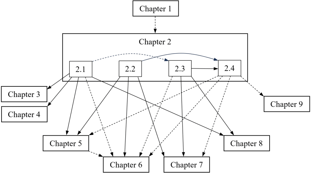
(I never learned how to make diagrams in LaTeX. You can usually do almost as well in Microsoft Word, with way less effort!)

 

Chapter 1: Introduction

“Algorithmic Bayesian epistemology” (the title of the thesis, a.k.a. ABE) just means “reasoning about uncertainty under constraints”. You might’ve seen math problems that look like this:

0.1% of people have a disease. You get tested using a test that’s ten times more likely to come up positive for people who have the disease than for people who don’t. If your test comes up positive, what’s the probability that you have the disease?

But the real world is rarely so simple: maybe there’s not one test but five. Test B is more likely to be a false positive in cases where Test A is a false positive. Tests B and C test for different sub-types for the disease, so they complement each other. Tests D and E are brand new and it’s unclear how correlated they are with the other tests. How do you form beliefs in that sort of information landscape?

Here’s another example. A month ago, I was deciding whether to change my solar eclipse travel plans from Mazatlán, Mexico to Montreal, Canada, on account of the weather forecasts. The American model told me that there was a 70% chance that it would be cloudy in Mazatlán; meanwhile, the Canadian model forecast a mere 20% chance. How was I to reconcile these sharply conflicting probabilities?^[2]

I was facing an informational constraint. Had I known more about the processes by which the models arrived at their probabilities and what caused them to diverge, I would have been able to produce an informed aggregate probability. But I don’t have that information. All I know is that it’s cloudy in Mazatlán 25 percent of the time during this part of the year, and that one source predicts a 20% chance of clouds while another predicts a 70% chance. Given just this information, what should my all-things-considered probability be?

(If you’re interested in this specific kind of question, check out Chapter 7 [LW · GW]!)

But informational constraints aren’t the only challenge. You can face computational constraints (you could in theory figure out the right probability, but doing so would take too long), or communicational constraints (figuring out the right probability involves talking to an expert with a really detailed understanding of the problem, but they only have an hour to chat), or strategic constraints (the information you need is held by people with their own incentives who will decide what to tell you based on their own strategic considerations).

So that’s the unifying theme of my thesis: reasoning about uncertainty under a variety of constraints.^[3]

I don’t talk about computational constraints very much in my thesis. Although that topic is really important, it’s been studied to death, and making meaningful progress is really difficult. On the other hand, some of the other kinds of constraints are really underexplored! For example, there’s almost no work on preventing strategic experts from colluding (Chapter 4 [LW · GW]), very little theory on how best to aggregate experts’ forecasts (Chapters 5 [LW · GW], 6 [LW · GW], 7 [LW · GW]), and almost no work on communicational constraints (Chapter 8 [LW · GW]). In no small part, I chose which topics to study based on where I expected to find low-hanging fruit.

 

Chapter 2: Preliminaries

This is a great chapter to read if you want to get a sense of what sort of stuff my thesis is about. It describes the foundational notions and results that the rest of my thesis builds on. Contents include:

• Proper scoring rules: suppose I want to know the probability that OpenAI will release GPT-5 this year. I could pay my friend Jaime at Epoch AI for a forecast. But how do I make sure that the forecast he gives me reflects his true belief? One approach is to ask Jaime for a forecast, wait to see if GPT-5 is released this year, and then pay him based on the accuracy of his forecast. Such a payment scheme is called a scoring rule, and we say that a scoring rule is proper if it actually incentivizes Jaime to report his true belief (assuming that he wants to maximize the expected value of his score). (I’ve written about proper scoring rules before on this blog! Reading that post might be helpful for understanding the rest of this one.)
• Forecast aggregation methods: now let’s say that Jaime thinks there’s a 40% chance that GPT-5 will be released this year, while his colleagues Ege and Tamay think there’s a 50% and 90% chance, respectively. What’s the right way for them to aggregate their probabilities into a single consensus forecast? One natural approach is to just take the average, but it turns out that there are significantly better approaches.
• Information structures: if some experts are interested in forecasting a quantity, an information structure is a way to formally express all of the pieces of information known by at least one of the experts, and how those pieces of information interact/overlap. I also discuss some “nice” properties that information structures can have, which make them easier to work with.

 

Chapter 3: Incentivizing precise forecasts

(Joint work with George Noarov and Matt Weinberg.)

I’ve actually written about this chapter of my thesis on my blog, so I’ll keep this summary brief!

In the previous section, I mentioned proper scoring rules: methods of paying an expert for a probabilistic forecast (depending on the forecast and the eventual outcome) in a way that incentivizes the expert to tell you their true probability.

The two most commonly used ones are the quadratic scoring rule (you pay the expert some fixed amount, and then subtract from that payment based on the expert’s squared error) and the logarithmic scoring rule (you pay the expert the log of the probability that they assign to the eventual outcome). (See this post or Chapter 2.1 of my thesis for a more thorough exposition.) But there are also infinitely many other proper scoring rules. How do you choose which one to use?

All proper scoring rules incentivize and expert to give an accurate forecast (by definition). In this chapter, I explore the question of which proper scoring rule most incentivizes an expert to give a precise forecast — that is, to do the most research before giving their forecast. Turns out that the logarithmic scoring rule is very good at this (99% of optimal), but you can do even better!

(Click here for my old blog post summarizing this chapter!)

 

Chapter 4: Arbitrage-free contract functions

(Joint work with my PhD advisor, Tim Roughgarden.)

Now let’s say that you’re eliciting forecasts from multiple experts. We can revisit the example I gave earlier: Jaime, Ege, and Tamay think there’s a 40%, 50%, and 90% chance that GPT-5 will be released this year. (These numbers are made up.)

Let’s say that I want to pay Jaime, Ege, and Tamay for their forecasts using the quadratic scoring rule. To elaborate on what this means, the formula I’ll use is: $100\cdot (1-(\text{forecasting error}{)}^2)$. For example, Jaime forecast a 40% chance. If GPT-5 is released this year, then the “perfect” forecast would be 100%, which means that his “forecasting error” would be 0.6. Thus, I would pay Jaime $\$100(1-{0.6}^2)=\$64$. On the other hand, if GPT-5 is not released, then his forecasting error would be 0.4, so I would pay Jaime $\$100(1-{0.4}^2)=\$84$.

To summarize all these numbers in a chart:

Expert	Forecast	Payment if YES	Payment if NO
Jaime	40%	$64	$84
Ege	50%	$75	$75
Tamay	90%	$99	$19
Total payment		$238	$178
Table 4.1: How much I owe to each expert under the YES outcome (GPT-5 is released this year) and the NO outcome (it’s not released this year).

But now, suppose that Jaime, Ege, and Tamay talk to each other and decide to all report the average of their forecasts, which in this case is 60%.

Expert	Forecast	Payment if YES	Payment if NO
Jaime	60%	$84	$64
Ege	60%	$84	$64
Tamay	60%	$84	$64
Total payment		$252	$192
Table 4.2: How much I owe to each expert under the YES and NO outcomes, if all three experts collude to say the average of their true beliefs.

In this case, I will owe more total dollars to them, no matter the outcome! They know this, and it gives them an opportunity to collude:

• Step 1: They all report the average of their beliefs (60%).
• Step 2: They agree to redistribute their total winnings in a way that leaves each of them better off than if they haven’t colluded. (For example, they could agree that if YES happens, they’ll redistribute the $252 so that Jaime gets $68, Ege gets $80, and Tamay gets $104, and if NO happens, they’ll redistribute the $192 so that Jaime gets $88, Ege gets $80, and Tamay gets $24.)

The collusion benefits them no matter what! Naturally, if I want to get an accurate sense of what each one of them believes, if I want to figure out how to pay them so that there’s no opportunity for them to collude like that.

And so there’s a natural question: is it possible to pay each expert in a way that incentivizes each expert to report their true belief and that prevents any opportunity for collusion? This question was asked in 2011 by Chun & Shachter.

In this chapter, I resolve Chun & Shachter’s question: yes, preventing Jaime, Ege, and Tamay from colluding is possible.

Why should this be possible? It’s because I can pit Jaime, Ege, and Tamay against each other. If there were only one expert, I could only reward the expert as a function of their own forecast. But if there are three experts, I can reward Jaime based on how much better his forecast was than Ege’s and Tamay’s. That’s the basic idea; if you want the details, go read Chapter 4!

 

* Chapter 5: Quasi-arithmetic pooling

(Joint work with my PhD advisor, Tim Roughgarden.)

As before, let’s say that I elicit probabilistic forecasts from Jaime, Ege, and Tamay using a proper scoring rule.^[4] How should I combine their numbers in a single, all-things-considered forecast?

In this chapter, I make the case that the answer should depend on the scoring rule that you used to elicit their forecasts.

To see why, consider for comparison the quadratic and logarithmic scoring rules. Here’s a plot of the score of an expert as a function of the probability they report, if the event ends up happening.

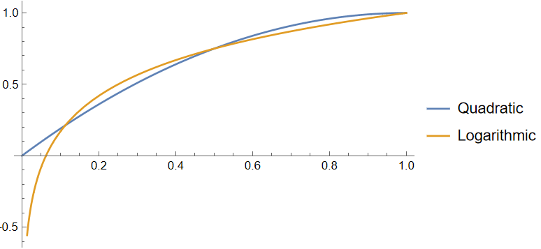
If Jaime says that there’s a 50% chance that GPT-5 comes out this year, and it does come out, he’ll get a score of 0.75 regardless of whether I use the quadratic or the log score. But if Jaime says that there’s a 1% chance that GPT-5 comes out this year, and it does come out, then he’ll get a score of 0.02 if I use the quadratic score, but will get a score of -0.66 if I use the log score.

(The scoring rules are symmetric: for example, Jaime’s score if predicts 30% and GPT-5 doesn’t come out is the same as if he had predicted 70% and it did come out.)

This means that Jaime cares which outcome happens a different amount depending on which scoring rule I use. Below is a plot of how much higher a score Jaime would get if GPT-5 did come out compared to if it didn’t, as a function of the probability that he reports.

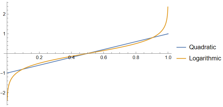
Suppose that Jaime reports an extreme probability, like 1% or 99%. This plot shows that Jaime cares much more about the outcome if I use the log score rule to reward him than if I use the quadratic score. This makes sense, since the log scoring rule is strongly punishes assigning a really low probability to the eventual outcome. But conversely, if Jaime reports a non-extreme probability, like 25% or 75%, he actually cares more about the outcome if I use the quadratic score than if I use the log score.

Intuitively, this means that if I use the log score, then Jaime cares a lot more about making his forecasts precise when they’re near the extremes. He cares about the difference between a 1% chance and a 0.1% chance, to a much greater degree than if I used the quadratic score. Jaime will think carefully and make his forecast extra precise before reporting a probability like 0.1%.

And so, if I use the log score and Jaime tells me 0.1% anyway, it makes sense for me to take that forecast seriously. If a different expert tells me 50%, it doesn’t make much sense for me to just take the average — 25.05% — because Jaime’s 0.1% forecast likely reflects a more informed, precise understanding.

To formalize this intuition, I came up with a method of aggregating forecasts that I called quasi-arithmetic pooling (QA pooling) with respect to the scoring rule being used for elicitation. Roughly speaking, instead of averaging the forecasted probabilities, QA pooling averages the kinds of numbers represented in Figure 5.2: each expert’s “amount of investment” in the possible outcomes. I was able to prove a bunch of cool properties of QA pooling:

• QA pooling with respect to the quadratic scoring rule just means taking the average of the forecasts (this is called linear pooling). QA pooling with respect to the logarithmic scoring rule involves treating the forecasts as odds instead of probabilities, and then taking their geometric mean (this is called logarithmic pooling). Logarithmic pooling is the second most well-studied forecast aggregation technique (after linear pooling), and it works very well in practice [EA · GW]. Thus, QA pooling maps the two most widely-used proper scoring rules to the two most well-studied forecast aggregation techniques!
• Suppose that your receive a bunch of forecasts from different experts. You don’t know the eventual outcome, but your goal is to beat the average of all the experts’ scores no matter which outcome happens, and by as much as possible in the worst case. The way to do that is to use QA pooling with respect to the scoring rule.
  • There’s a natural interpretation of this fact in terms of the concept of the wisdom of crowds. Suppose a bunch of people (the crowd) report forecasts. Is it possible to do better that a single random crowd member — that is, to guarantee yourself a better score than the average person in the crowd? The answer is yes! And the way to beat the crowd by the largest possible amount is to QA-pool the forecasts. In that sense, the QA pool is the correct way to aggregate the crowd (with respect to whichever scoring rule you care about). On this view, “wisdom of the crowds” is not just an empirical fact, but a mathematical one!
• You can also do QA pooling with different weights for different experts (just like you can take a weighted average of numbers instead of a simple average). This is useful if you trust some experts more than others. But how can you decide how much to trust each expert? It turns out that so long as the scoring rule is bounded (e.g. quadratic, but not log), you can learn weights for experts over time based on the experts’ performance, and you’ll do almost as well as if you had known the best possible weights from the get-go. (In the field of online learning, this is called a no-regret algorithm.)
• QA pooling can be used to define what it means to be over- or under-confident. This notion of overconfidence turns out to be equivalent to another natural notion of overconfidence (one that I first came up with in order to analyze the results of my pseudorandomness contest).
• When coming up with a method of aggregating forecasts, there are some axioms/desiderata that you might want your aggregation method to satisfy. It turns out that for a certain natural set of axioms, the class of aggregation methods that comply with those axioms is precisely the class of all QA pooling methods.

In all of these senses, QA pooling seems like a really natural way to aggregate forecasts. I’m really excited to see QA pooling investigated further!

 

Chapter 6: Learning weights for logarithmic pooling

(Joint work with my PhD advisor, Tim Roughgarden.)

In my description of Chapter 5, I said:

It turns out that so long as the scoring rule is bounded (e.g. quadratic, but not log), you can learn weights for experts over time based on the experts’ performance, and you’ll do almost as well as if you known the best possible weights from the get-go.

That is fair enough, but many natural proper scoring rules (such as the log score) are in fact unbounded. It would be nice to have results in those cases as well.

Unfortunately, if the scoring rule is unbounded, there is no way to get any result like this unconditionally. In particular, if your experts are horribly miscalibrated (e.g. if 10% of the time, they say 0.00000001% and then the event happens anyway), there’s no strategy for putting weights on the experts that can be guaranteed to work well.

But what if you assume that the experts are actually calibrated? In many cases, that’s a pretty reasonable assumption: for example, state-of-the-art machine learning systems are calibrated. So if you have a bunch of probability estimates from different AIs and you want to aggregate those estimates into a single number (this is called “ensembling”), it’s pretty reasonable to make the assumption that the AIs are giving you calibrated probabilities.

In this chapter, I prove that at least for the log scoring rule, you can learn weights for experts over time in a way that’s guaranteed to perform well on average, assuming that the experts are calibrated. (For readers familiar with online learning: the algorithm is similar to online mirror descent with a Tsallis entropy regularizer.)

 

* Chapter 7: Robust aggregation of substitutable signals

(Joint work with my PhD advisor, Tim Roughgarden.)

Let’s say that it rains on 30% of days. You look at two (calibrated) weather forecasts: Website A says there’s a 60% chance that it’ll rain tomorrow, while Website B says there’s a 70% chance. Given this information, what’s your all-things-considered estimate of how likely it is to rain tomorrow?

The straightforward answer to this question is that I haven’t given you enough information. If Website A’s is strictly more informed than Website B, you should say 60%. If Website B is strictly more informed than Website A, you should say 70%. If the websites have non-overlapping information, you should say something different than if their information is heavily overlapping. But I haven’t told you that, so I haven’t given you the information you need in order to produce the correct aggregate forecast.

In my opinion, that’s not a good excuse, because often you lack this information in practice. You don’t know which website is more informed and by how much, or how much their information overlaps. Despite all that, you still want an all-things-considered guess about how likely it is to rain. But is there even a theoretically principled way to make such a guess?

In this chapter, I argue that there is a principled way to combine forecasts in the absence of this knowledge, namely by using whatever method works as well as possible under worst-case assumptions about how the experts’ information sets overlap. This is a quintessentially theoretical CS-y way of looking at the problem: when you lack relevant information, you pick a strategy that’ll do well robustly, i.e. no matter what that information happens to be. In other words: you want to guard as well as possible against nasty surprises. This sort of work has been explored before under the name of robust forecast aggregation — but most of that work has had to make some pretty strong assumptions about the forecasters’ information overlap (for example, that there are two experts, one of whom is strictly more informed than the other, but you don’t know which).

By contrast, in this chapter I make a much weaker assumption: roughly speaking, all I assume is that the experts’ information is substitutable, in the economic sense of the word. This means that there’s diminishing marginal returns to learning additional experts’ information. This is a natural assumption that holds pretty often: for example, suppose that Website A knows tomorrow’s temperature and cloud cover, whereas Website B knows tomorrow’s temperature and humidity. Since their information overlaps (they both know the temperature), Website B’s information is less valuable if you already know Website A’s information, and vice versa.

 

The chapter has many results: both positive ones (“if you use this strategy, you’re guaranteed to do somewhat well”) and negative ones (“on the other hand, no strategy is guaranteed to do very well in the worst case”). Here I’ll highlight the most interesting positive result, which I would summarize as: average, then extremize.

In the leading example, I gave two pieces of information:

• Each expert’s forecast (60% and 70%)
• The prior — that is, the forecast that someone with no special information would give (30%)

A simple heuristic you might use is to average the experts’ forecasts, ignoring the prior altogether: after all, the experts know that it rains on 30% of days, and they just have some additional information.

Yet, the fact that the experts updated from the prior in the same direction is kind of noteworthy. To see what I mean, let’s consider a toy example. Suppose that I have a coin, and I have chosen the coin’s bias (i.e. probability of coming up heads) uniformly between 0% and 100%. You’re interested in forecasting the bias of the coin. Since I’ve chosen the bias uniformly, your best guess (without any additional information) is 50%.

Now, suppose that two forecasters each see an independent flip of the coin. If you do the math, you’ll find that if a forecasters sees heads, they should update their guess for the bias to 2/3, and if they see tails, they should update to 1/3. Let’s say that both forecasters tell you that their guess for the bias of the coin is 2/3 — so you know that they both saw heads. What should your guess be about the bias of the coin?

Well, you now have more information that either forecaster: you know that the coin came up heads both times it was flipped! And so you should actually say 3/4, rather than 2/3. That is, because the two forecasters saw independent evidence that pointed in the same direction, you should update even more in that direction. This move — updating further away from the prior after aggregating the forecasts you have available — is called extremization.

Now, generally speaking, experts’ forecasts won’t be based on completely independent information, and so you won’t want to extremize quite as much as you would if you assumed independence. But as long as there’s some non-overlap in the experts’ information, it does make sense to extremize at least a little.

The benefits to extremization aren’t just theoretical: Satopää et al. found that extremization improves aggregate forecasts, and Jaime Sevilla found that [EA · GW] the extremization technique I suggest in this chapter works well on data from the forecast aggregator Metaculus.

 

Beyond giving a theoretical grounding to some empirical results in forecast aggregation, I’m excited about the work in this chapter because it opens up a whole bunch of new directions for exploration. Ultimately, in this chapter I made progress on a pretty narrow question. I won’t define all these terms, but here’s the precise question I answered:

What approximation ratio can be achieved by an aggregator who learns expected value estimates of a real-valued quantity Y from m truthful experts whose signals are drawn from an information structure that satisfies projective substitutes, if the aggregator’s loss is their squared error and the aggregator knows nothing about the information structure or only knows the prior?

Each of the bolded clauses can be varied. Relative to what baseline do we want to measure the aggregator’s performance? What sort of information does the aggregator get from the experts? Are the experts truthful or strategic? What assumptions are we making about the interactions between the experts’ information? What scoring rule are we using to evaluate the forecasts? In all, there are tons of different questions you can ask within the framework of robust forecast aggregation. I sometimes imagine this area as a playground with a bunch of neat problems that people have only just started exploring. I’m excited!

 

Chapter 8: When does agreement imply accuracy?

(Joint work with Raf Frongillo and Bo Waggoner.)

In 2005, Scott Aaronson wrote one of my favorite papers ever: The Complexity of Agreement. (Aaronson’s blog post summarizing the paper, which I read in 2015, was a huge inspiration and may have been counterfactually responsible for my thesis!) Here’s how I summarize Aaronson’s main result in my thesis:

Suppose that Alice and Bob are honest, rational Bayesians who wish to estimate some quantity — say, the unemployment rate one year from now. Alice is an expert on historical macroeconomic trends, while Bob is an expert on contemporary monetary policy. They convene to discuss and share their knowledge with each other until they reach an agreement about the expected value of the future unemployment rate. Alice and Bob could reach agreement by sharing everything they had ever learned, at which point they would have the same information, but the process would take years. How, then, should they proceed?

In the seminal work “Agreeing to Disagree,” Aumann (1976) observed that Alice and Bob can reach agreement simply by taking turns sharing their current expected value for the quantity[…] A remarkable result by Aaronson (2005) shows that if Alice and Bob follow certain protocols of this form, they will agree to within with probability by communicating bits [of information…] Notably, this bound only depends on the error Alice and Bob are willing to tolerate, and not on the amount of information available to them.

In other words: imagine that Alice and Bob — both experts with deep but distinct knowledge — have strongly divergent opinions on some topic, leading them to make different predictions. You may have thought that Alice and Bob would need to have a really long conversation to hash out their differences — but no! At least if we model Alice and Bob as truth-seeking Bayesians, they can reach agreement quite quickly, simply by repeatedly exchanging their best guesses: first, Alice tells Bob her estimate. Then, Bob updates his estimate in light of the estimate he just heard from Alice, and responds with his new estimate. Then, Alice updates her estimate in light of the estimate he just heard from Bob, and responds with her new estimate. And so on. After only a small number of iterations, Alice and Bob are very likely to reach agreement!^[5]

However, while Aaronson’s paper shows that Alice and Bob agree, there’s no guarantee that the estimate that they agree on is accurate. In other words, you may have hoped that by following Aaronson’s protocol (i.e. repeatedly exchanging estimates until agreement is reached), the agreed-upon estimate would be similar to the estimate that Alice and Bob would have reached if they had exchanged all of their information. Unfortunately, no such accuracy guarantee is possible.

As a toy example, suppose that Alice and Bob each receive a random bit (0 or 1) and are interested in estimating the XOR of their bits (that is, the sum of their bits modulo 2).

	Bob’s bit = 0	Bob’s bit = 1
Alice’s bit = 0	XOR = 0	XOR = 1
Alice’s bit = 1	XOR = 1	XOR = 0
Table 8.2: XOR

Since Alice knows nothing about Bob’s bit, she thinks there’s a 50% chance that his bit is the same as hers and a 50% chance that his bit is different from hers. This means that her estimate of the XOR is 0.5 from the get-go. And that’s also Bob’s estimate — which means that they agree from the start, and no communication is necessary to reach agreement. Alas, 0.5 is very far from the true value of the XOR, which is either 0 or 1.

In this example, even though Alice and Bob agreed from the start, their agreement was superficial: it was based on ignorance. They merely agreed because the information they had was useless in isolation, and only informative when combined together. Put otherwise, to an external observer, finding out Bob’s bit is totally useless without knowing Alice’s bit, but extremely useful if they already know Alice’s bit. Alice and Bob’s pieces of information are complements rather than substitutes. (Recall also that the notion of informational substitutes came up in Chapter 7!)

This observation raises a natural question: what if we assume that Alice and Bob’s information is substitutable — that is, an external observer gets less mileage from learning Bob’s information if they already know Alice’s information, and vice versa? In that case, are Alice and Bob guaranteed to have an accurate estimate as soon as they’ve reached agreement?

In this chapter, I show that the answer is yes! There’s a bunch of ways to define informational substitutes, but I give a particular (admittedly strong) definition under which agreement does imply accuracy.

I’m excited about this result for a couple reasons. First, it provides another example of substitutes-like conditions on information being useful (on top of the discussion in Chapter 7 [LW · GW]). Second, the result can be interpreted in the context of prediction markets. In a prediction market, participants don’t share information directly; rather, they buy and sell shares, thus partially sharing their beliefs about the expected value of the quantity of interest. Thus, this chapter’s main result might also shed light on the question of market efficiency: under what conditions does the price of a market successfully incorporate all traders’ information into the market price? This chapter’s suggested answer: when the traders’ pieces of information are substitutable, rather than complementary.^[6]

I generally think that the topic of agreement — and more generally, communication-constrained truth-seeking — is really neglected relative to how interesting it is, and I’d be really excited to see more work in this direction.

 

* Chapter 9: Deductive circuit estimation

(Joint work at the Alignment Research Center with Paul Christiano, Jacob Hilton, Václav Rozhoň, and Mark Xu.)

This chapter is definitely the weirdest of the bunch. It may also be my favorite.

A boolean circuit is a simple kind of input-output machine. You feed it a bunch of bits (zeros and ones) as input, it performs a bunch of operations (ANDs, ORs, NOTs, and so forth), and outputs — for the purposes of this chapter — a single bit, 0 or 1. Boolean circuits are the building blocks that computers are made of.

Let’s say that I give you a boolean circuit C. How would you go about estimating the fraction of inputs on which C will output 1? (I call this quantity C’s acceptance probability, or p(C).) The most straightforward answer is to sample a bunch of random inputs and then just check what fraction of them cause C to output 1.

This is very effective and all, but it has a downside: you’ve learned nothing about why C outputs 1 as often as it does. If you want to understand why a circuit outputs 1 on 99% of inputs, you can’t just look at the input-output behavior: you have to look inside the circuit and examine its structure. I call this process deductive circuit estimation, because it uses deductive reasoning, as opposed to sampling-based estimation (which uses inductive reasoning). Deductive reasoning of this kind is based on “deductive arguments”, which point out something about the structure of a circuit in order to argue about the circuit’s acceptance probability.

Here are a few examples, paraphrased from the thesis:

Suppose that a circuit C takes as input a triple (a, b, c) of positive integers (written down in binary). It computes max(a, b) and max(b, c), and outputs 1 if they are equal. A deductive argument about C might point out that if b is the largest of the three integers, then max(a, b) = b = max(b, c), and so C will output 1, and that this happens with probability roughly 1/3.

This argument points out that C outputs 1 whenever b is the largest of the three integers. The argument does not point out that C also outputs 1 when a and c are both larger than b and happen to be equal. In this way, deductive arguments about circuits can help distinguish between different “reasons why” a circuit might output 1. (More on this later.)

The next example makes use of SHA-256, which is a famous hash function: the purpose of SHA-256 is to produce “random-looking” outputs that are extremely hard to predict.

Suppose that C(x) computes SHA-256(x) (the output of SHA-256 is a 256-bit string) and outputs 1 if the first 128 bits (interpreted as an integer) are larger than the last 128 bits. One can make a deductive argument about p(C) by making repeated use of the presumption of independence. In particular, the SHA-256 circuit consists of components that produce uniformly random outputs on independent, uniformly random inputs. Thus, a deductive argument that repeatedly presumes that the inputs to each component are independent concludes that the output of SHA-256 consists of independent, uniformly random bits. It would then follow that the probability that the first 128 bits of the output are larger than the last 128 bits is 1/2.

The third example is about a circuit that checks for twin primes. This example points out that deductive arguments ought to be defeasible: a deductive argument can lead you to an incorrect estimate of p(C), but in that case there ought to be a further argument about C that will improve your estimate.

Suppose that C takes as input a random integer k between and and accepts if k and k + 2 are both prime. A deductive argument about p(C) might point out that the density of primes in this range is roughly 1%, so if we presume that the event that k is prime and the event that k + 2 is prime are independent, then we get an estimate of p(C) = 0.01%. A more sophisticated argument might take this one step further by pointing out that if k is prime, then k is odd, so k + 2 is odd, which makes k + 2 more likely to be prime (by a factor of 2), suggesting a revised estimate of p(C) = 0.02%. A yet more sophisticated argument might point out that additionally, if k is prime, then k is not divisible by 3, which makes k + 2 more likely to be divisible by 3, which reduces the chance that k + 2 is prime.

In this chapter, I ask the following question: is there a general-purpose deductive circuit estimation algorithm, which takes as input a boolean circuit C and a list of deductive arguments about C, and outputs a reasonable estimate of p(C)? You can think of such an algorithm as being analogous to a program that verifies formal proofs. Much as a proof verifier takes as input a mathematical statement and a purported formal proof, and accepts if the proof actually proves the statement, a deductive circuit estimator takes as input a circuit together with observations about the circuit, and outputs a “best guess” about the circuit’s acceptance probability. A comparison table from the thesis:

Deductive circuit estimation	Formal proof verification
Deductive estimation algorithm	Proof verifier
Boolean circuit	Formal mathematical statement
List of deductive arguments	Alleged proof of statement
Formal language for deductive arguments	Formal language for proofs
Desiderata for estimation algorithm	Soundness and completeness
Algorithm’s estimate of circuit’s acceptance probability	Proof verifier’s output (accept or reject)
Table 9.1: We are interested in developing a deductive estimation algorithm for boolean circuits. There are similarities between this task and the (solved) task of developing an algorithm for verifying formal proofs of mathematical statements. This table illustrates the analogy. Importantly, the purpose of a deductive estimation algorithm is to incorporate the deductive arguments that it has been given as input, rather than to generate its own arguments. The output of a deductive estimation algorithm is only as sophisticated as the arguments that it has been given.

Designing a deductive estimation algorithm requires you to do three things:

1. Come up with a formal language in which deductive arguments like the ones in the above examples can be expressed.
2. Come up with a list of desiderata (i.e. “reasonableness properties”) that the deductive estimation algorithm ought to satisfy.
3. Find an algorithm that satisfies those desiderata.

In this chapter, I investigate a few desiderata:

• Linearity: given a circuit C with input bits $x_1,\dots ,x_n$, define $C[x_i=0]$ to be the circuit that you get when you “force” $x_i$ to be 0. (The resulting circuit now has n – 1 inputs instead of n.) Define $C[x_i=1]$ analogously. The deductive estimator’s estimate of p(C) should be equal to the average of its estimate of $p\left(C\right[x_i=0\left]\right)$ and $p\left(C\right[x_i=1\left]\right)$.
• Respect for proofs: a formal proof that bounds the value of p(C) can be given to the deductive estimator as an argument, and forces the deductive estimator to output an estimate that’s within that bound.
• 0-1 boundedness: the deductive estimator’s estimate of the acceptance probability of any circuit is always between 0 and 1.

In this chapter, I give an efficient algorithm that satisfies the first two of these properties. The algorithm is pretty cool, but I argue that ultimately it isn’t what we’re looking for, because it doesn’t satisfy a different (informal) desirable property called independence of irrelevant arguments. That is, the algorithm I give produces estimates that can be easily influenced by irrelevant information.

Does any efficient algorithm satisfy all three of the linearity, respect for proofs, and 0-1 boundedness? Unfortunately, the answer is no (under standard assumptions from complexity theory). However, I argue that 0-1 boundedness isn’t actually that important to satisfy, and that instead we should be aiming to satisfy the first two properties along with some other desiderata. I discuss what those desiderata may look like, but ultimately leave the question wide open.

 

Even though this chapter doesn’t get close to actually providing a good algorithm for deductive circuit estimation, I’m really excited about it, for two reasons.

The first reason is that I think this problem is objectively really cool and arguably fundamental. Just as mathematicians formalized the notion of a mathematical proof a century ago, perhaps this line of work will lead to a formalization of a much broader class of deductive arguments.

The second reason for my excitement is because of potential applications to AI safety. When we train an AI, we train it to produce outputs that look good to us. But one of the central difficulties of building safe advanced AI systems is that we can’t always tell whether an AI output looks good because it is good or because it’s bad in a way we don’t notice. A particularly pernicious failure mode is when the AI intentionally tricks us into thinking that its output was good.

(Consider a financial assistant AI that takes actions like buying and selling stocks, transferring money between bank accounts, and paying taxes, and suppose we train the AI to turn a profit, subject to passing some basic checks for legal compliance. If the AI finds a way to circumvent the compliance checks — e.g. by doing some sophisticated, hard-to-notice money laundering — then it could trick its overseers into thinking that it’s doing an amazing job, despite taking actions that the overseers would strongly disapprove of if they knew about them.)

How does this relate to deductive circuit estimation? Earlier I mentioned that deductive arguments can let you distinguish between different reasons why a circuit might exhibit some behavior (like outputting 1). Similarly, if we can formally explain the reasons why an AI exhibits a particular behavior (like getting a high reward during training), then we can hope to distinguish between benign reasons for that behavior (it did what we wanted) and malign reasons (it tricked us).

This is, of course, a very surface-level explanation (see here for a slightly more in-depth one), and there’s a long ways to go before the theory in this chapter can be put into practice. But I think that this line of research is one of the most promising for addressing some of the most pernicious ways in which AIs could end up being unsafe.

(I am now employed at the Alignment Research Center, and am really excited about the work that we’ve been doing — along these lines and others — to understand neural network behavior!)

 

Epilogue

As you can probably tell, I’m really excited about algorithmic Bayesian epistemology as a research direction. Partly, that’s because I think I solved a bunch of cool problems in some really under-explored areas. But I’m equally excited by the many questions I didn’t answer and areas I didn’t explore. In the epilogue, I discuss some of the questions that I’m most excited about:

• Bayesian justifications for generalized QA pooling: In Chapter 5 [LW · GW], I defined QA pooling as a particular way to aggregate forecasts that’s sensitive to the scoring rule that was used to elicit the forecasts. One natural generalization of QA pooling allows experts to have arbitrary weights that don’t need to add to 1. It turns out that for the quadratic and logarithmic scoring rules, this generalization has natural “Bayesian justifications”. This means that in some information environments, generalized linear and logarithmic pooling is the best possible way to aggregate experts’ forecasts. (See Section 2.4 for details.) I’m really curious whether there’s a Bayesian justification for generalized QA pooling with respect to every proper scoring rule.
• Directions in robust forecast aggregation: In Chapter 7 [LW · GW], I discussed robust forecast aggregation as a theoretically principled, “worst-case optimal” approach to aggregating forecasts. There are a whole bunch of directions in which one could try to generalize my results. For example, the work I did in that chapter makes the most sense in the context of real-valued forecasts (which don’t have to be between 0 and 1), and I’d love to see work along similar lines in the context of aggregating probabilities, with KL divergence used as the notion of error instead of squared distance.
• Finding a good deductive estimator: In Chapter 9 [LW · GW], I set out to find a deductive circuit estimation algorithm that could handle a large class of deductive arguments in a reasonable way. Ultimately I didn’t get close to finding such an algorithm, and I would love to see more progress on this.
• Sophisticated Bayesian models for forecast aggregation: While several of the chapters of my thesis were about forecast aggregation, none of them took the straightforwardly Bayesian approach of making a model of the experts’ information overlap. I have some ideas for what a good Bayesian model could look like, and I’d love to see some empirical work on how well the model would work in practice. (If this sounds up your alley, shoot me an email!)
• Wagering mechanisms that produce good aggregate forecasts: Wagering mechanisms are alternatives to prediction markets. In a wagering mechanism, forecasters place wagers in addition to making predictions, and those wagers get redistributed according to how well the forecasters did. These mechanisms haven’t been studied very much, and — as far as I know — have never been used in practice. That said, I think wagering mechanisms are pretty promising and merit a lot more study. In part, that’s because wagering mechanisms give an obvious answer to the question of “how much should you weigh each forecaster’s prediction”: proportionally to their wagers! But as far as I know, there’s no theorem saying this results in good aggregate forecasts. I would love to see a wagering mechanism and a model of information for which you could prove that equilibrium wagers result in good aggregate forecasts.

 

My thesis is called Algorithmic Bayesian Epistemology, and I’m proud of it.

 

 

Thanks so much to my thesis advisor, Tim Roughgarden. He was really supportive throughout my time in grad school, and was happy to let me explore whatever I wanted to explore, even if it wasn’t inside his area of expertise. That said, even though algorithmic Bayesian epistemology isn’t Tim’s focus area, his advice was still really helpful. Tim has a really expansive knowledge of essentially all of theoretical computer science, which means he was able to see connections and make suggestions that I wouldn’t have come up with myself.️️️️

1. ^{^}

   I don’t want to make the video of my defense public, but email me if you want to see it!

2. ^{^}

   The right answer, as far as I can tell, is to defer to the NWS’ National Blend of Models. But that just raises the question: how does the National Blend of Models reconcile disagreeing probabilities?

3. ^{^}

   How did the name “Algorithmic Bayesian Epistemology” come about? “Bayesian epistemology” basically just means using probabilities to reason about uncertainty. “Algorithmic” is more of a term of art, which in this case means looking for satisfactory solutions that adhere to real-world constraints, as opposed to solutions that would be optimal if you ignored those constraints. See here [LW · GW] for a longer explanation.

4. ^{^}

   Our discussion of collusion was confined to Chapter 4 — now we’re assuming the experts can’t collude and instead just tell me their true beliefs.

5. ^{^}

   Unfortunately, this protocol is only communication-efficient. To actually update their estimates, Alice and Bob may potentially need to do a very large amount of computation at each step.

6. ^{^}

   Interestingly, Chen and Waggoner (2017) showed that under a (different) informational substitutes condition, traders in a prediction market are incentivized reveal all of their information right away by trading. This question of incentives is different from the question of my thesis chapter: my chapter can be interpreted as making the assumption that traders will trade on their information, and asking whether the market price will end up reflecting all traders’ information. Taken together, these two results suggest that market dynamics may be quite nice indeed when experts have substitutable information!

4 comments

Comments sorted by top scores.