Toy Models of Feature Absorption in SAEs
post by chanind, hrdkbhatnagar, TomasD (tomas-dulka), Joseph Bloom (Jbloom) · 2024-10-07T09:56:53.609Z · LW · GW · 8 commentsContents
  TLDR;
  What is feature absorption?
  How is this different than traditional feature splitting?
  Why does absorption happen?
  How big of a problem is this, really?
  Toy Models of Feature Absorption Setup
    Non-superposition setup
    Superposition setup
  Perfect Reconstruction with Independent Features
  Feature co-occurrence causes absorption
  Magnitude variance causes partial absorption
    Why does partial absorption happen?
  Imperfect co-occurrence can still lead to absorption depending on L1 penalty
  Tying the SAE encoder and decoder weights solves feature absorption
  Absorption in superposition
  Tying the encoder and decoder weights still solves feature absorption in superposition.
  Future work
  Acknowledgements
None
8 comments
TLDR;
In previous work [LW · GW], we found a problematic form of feature splitting called "feature absorption" when analyzing Gemma Scope SAEs. We hypothesized that this was due to SAEs struggling to separate co-occurrence between features, but we did not prove this. In this post, we set up toy models where we can explicitly control feature representations and co-occurrence rates and show the following:
- Feature absorption happens when features co-occur.
- If co-occurring feature magnitudes vary relative to each other, we observe "partial absorption", where a latent tracking a main feature sometimes fires weakly instead of not firing at all, but sometimes does fully not fire.
- Feature absorption happens even with imperfect co-occurrence, depending on the strength of the sparsity penalty.
- Tying the SAE encoder and decoder weights together solves feature absorption in toy models.
All code for this post can be seen in this Colab notebook.
The rest of this post will assume familiarity with Sparse Autoencoders (SAEs). But first, some background on feature absorption:
What is feature absorption?
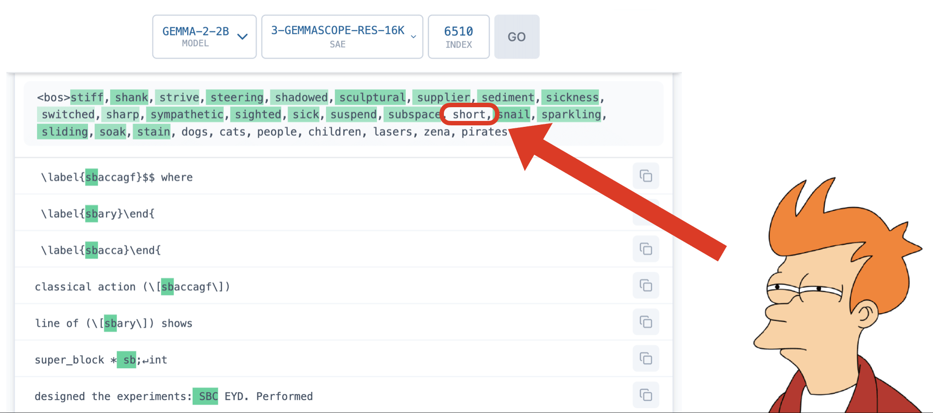
Feature absorption is a problematic form of feature splitting where a SAE latent appears to track an interpretable concept, but actually has holes in its recall. Instead, other SAE latents fire on specific tokens and "absorb" the feature direction into approximately token-aligned latents.
For instance, in Gemma Scope SAEs we find a latent which seems to track the feature that a token "starts with S". However, the latent will not fire on a few specific tokens that do start with S, like the token "short".
How is this different than traditional feature splitting?
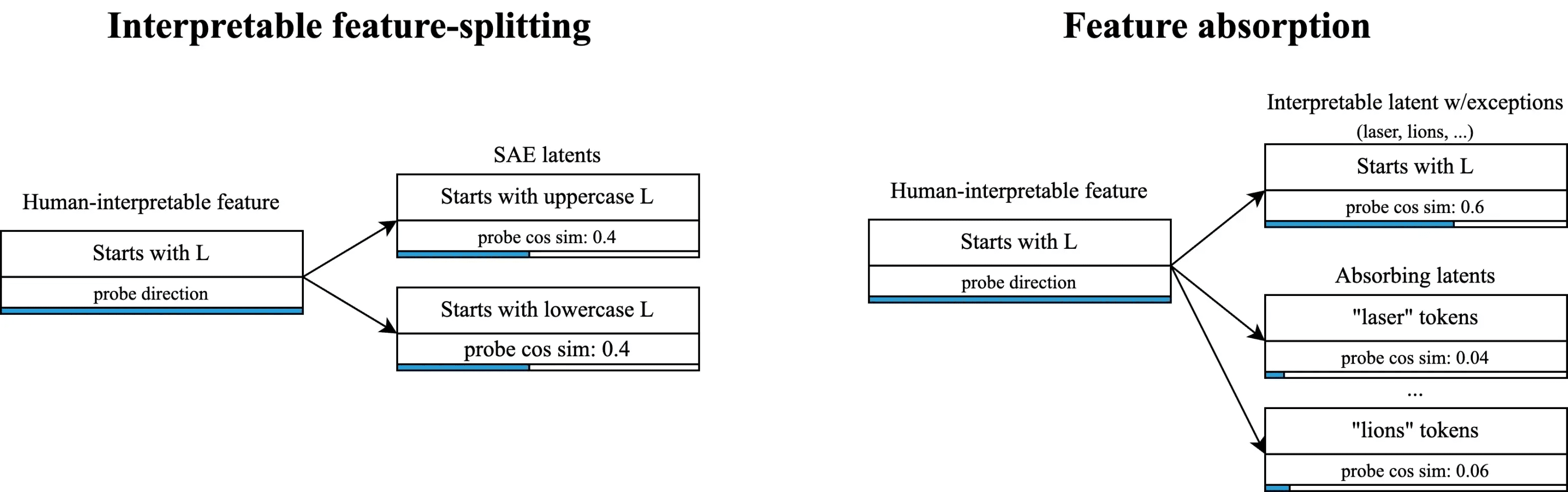
In traditional feature splitting, we expect a more general latent to split into more specific latent, but still tracking the same concept and still interpretable. For instance, a "starts with L" latent might split into "starts with uppercase L" and "stats with lowercase L". Theses more specific latents are still about starting with the letter L and nothing else, just more specific variants on it.
Traditional feature splitting doesn't pose a problem for interpretability. In fact, it may even be desirable to be able to control how fine or corse grained a SAE's latents are!
Feature absorption is different. In feature absorption, we end up with something like "Starts with L with a bunch of exceptions", and then we get combo latents like "lion" which encode both "lionness" and "starts with L".
Feature absorption strictly reduces interpretability, and makes it hard to trust that a feature is doing what is appears to be doing. This is especially problematic when we don't have ground truth labels, for instance if we're trusting a latent tracking "deception" by the model. Furthermore, absorption makes it SAEs significantly less useful as an interpretability technique, because it means latent directions are spreading "true feature directions" across a number of unrelated latents.
Why does absorption happen?
We hypothesized that absorption is due to feature co-occurrence combined with the SAE maximizing sparsity. When two features co-occur, for instance "starts with S" and "short", the SAE can increase sparsity by merging the "starts with S" feature direction into a latent tracking "short" and then simply not fire the main "start with S" latent. This means firing one feature instead of two! If you're an SAE, this is a big win.
How big of a problem is this, really?
Our investigation implies that feature absorption will happen any time features co-occur. Unfortunately co-occurrence is probably the norm rather than the exception. It's rare to encounter a concept that's fully disconnected from all other concepts, and occurs completely independently of everything else. Any time we can say "X is Y" about concepts X and Y that means that there's co-occurrence between these concepts. "dogs" are "animals"? co-occurrence. The "sky" is "blue"? co-occurrence. "3" is a "number"? co-occurrence. In fact, it's very difficult to think of any concept that doesn't have any relation to another concept like this.
Toy Models of Feature Absorption Setup
Following the example of "Toy Models of Superposition" and "Sparse autoencoders find composed features in small toy models [LW · GW]", we want to put together a simple test environment where we can control everything going on to understand exactly under what conditions feature absorption happens. We have two setups, one without superposition and one with superposition.
Non-superposition setup
Our initial setup consists of 4 true features, each randomly initialized into orthogonal directions with a 50 dimensional representation vector and unit norm, so there is no superposition. We control the base firing rates of each of the 4 true features. Unless otherwise specified, the feature fires with magnitude 1.0 and stdev 0.0. We train a SAE with 4 latents to match the 4 true features using SAELens. The SAE uses L1 loss with coefficient 3e-5, and learning rate 3e-4. We train on 100,000,000 activations. Our 4 true features have the following firing rates:
| Feature 0 | Feature 1 | Feature 2 | Feature 3 | |
|---|---|---|---|---|
| Firing rate | 0.25 | 0.05 | 0.05 | 0.05 |
We use this setup for several reasons:
- This is a very easy task for a SAE, and it should be able to reconstruct these features nearly perfectly.
- Using fully orthogonal features lets us see exactly what the L1 loss term incentivizes to happen without worrying about interference from superposition.
- This setup allows us to use exact same feature representations for each study in this post.
Regardless, most of these decisions are arbitrary, and we expect that the conclusions here should still hold for different choices of toy model setup.
Superposition setup
After we've demonstrated feature absorption in this simple setup and show that tying the SAE encoder and decoder together solves absorption, we then investigate the more complicated setup of superposition. In our superposition setup, we use 10 features each with a 9 dimensional representation. We randomly initialize these representations then optimize them to be as orthogonal as possible. We also increase the L1 loss term to 3e-2 as this seems to be necessary with more features in superposition. Otherwise, everything else is the same as in the non-superposition setup.
Perfect Reconstruction with Independent Features
When the true features fire independently, we find that the SAE is able to perfectly recover these features.
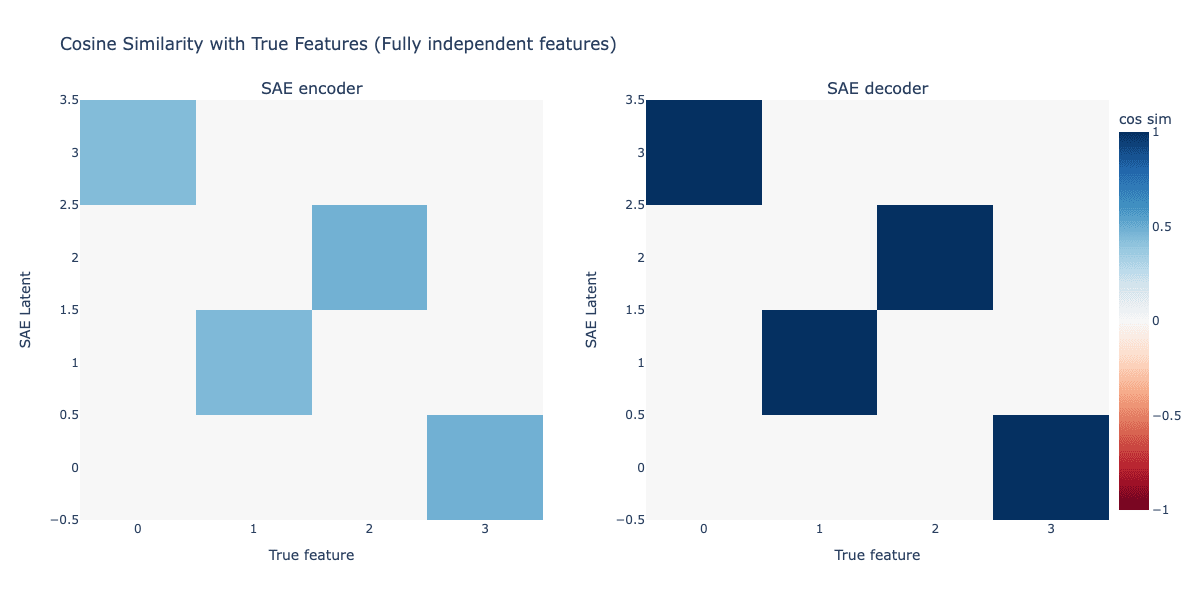
Above we see the cosine similarity between the true features and the learned encoder, and likewise with the true features and the decoder. The SAE learns one latent per true feature. The decoder representations perfectly match the true feature representations, and the encoder learns to perfectly segment out each feature from the other features. This is what we hope SAEs should do!
Feature co-occurrence causes absorption
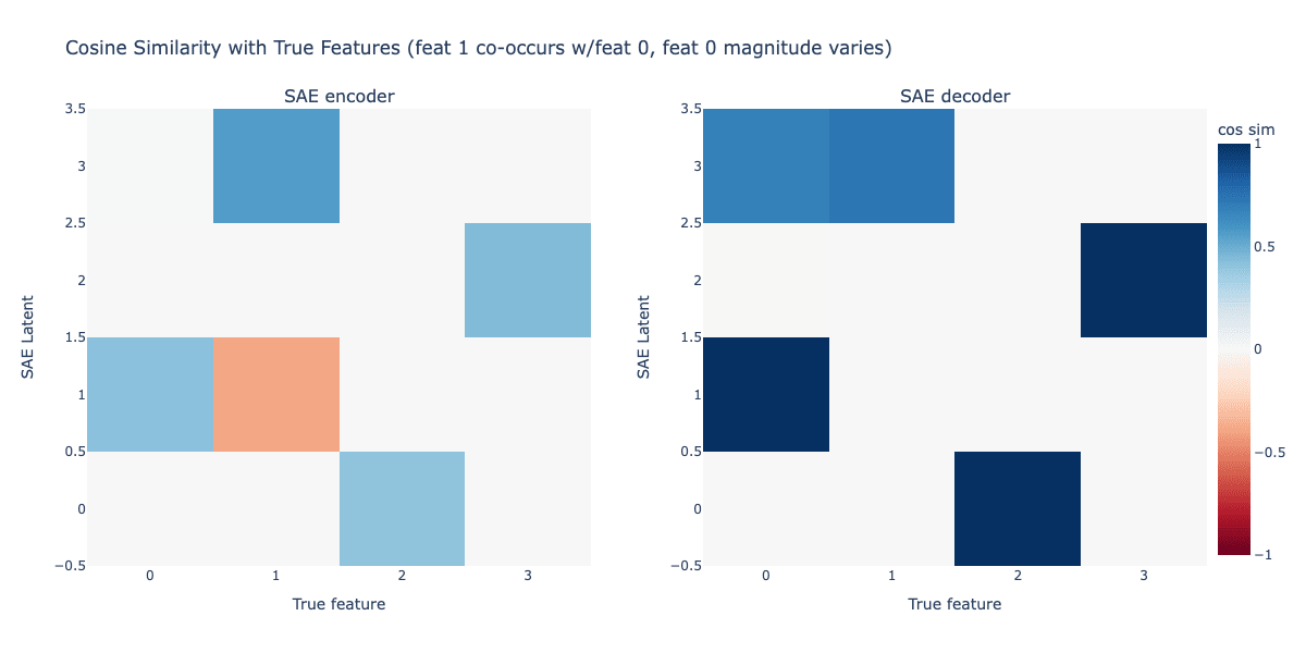
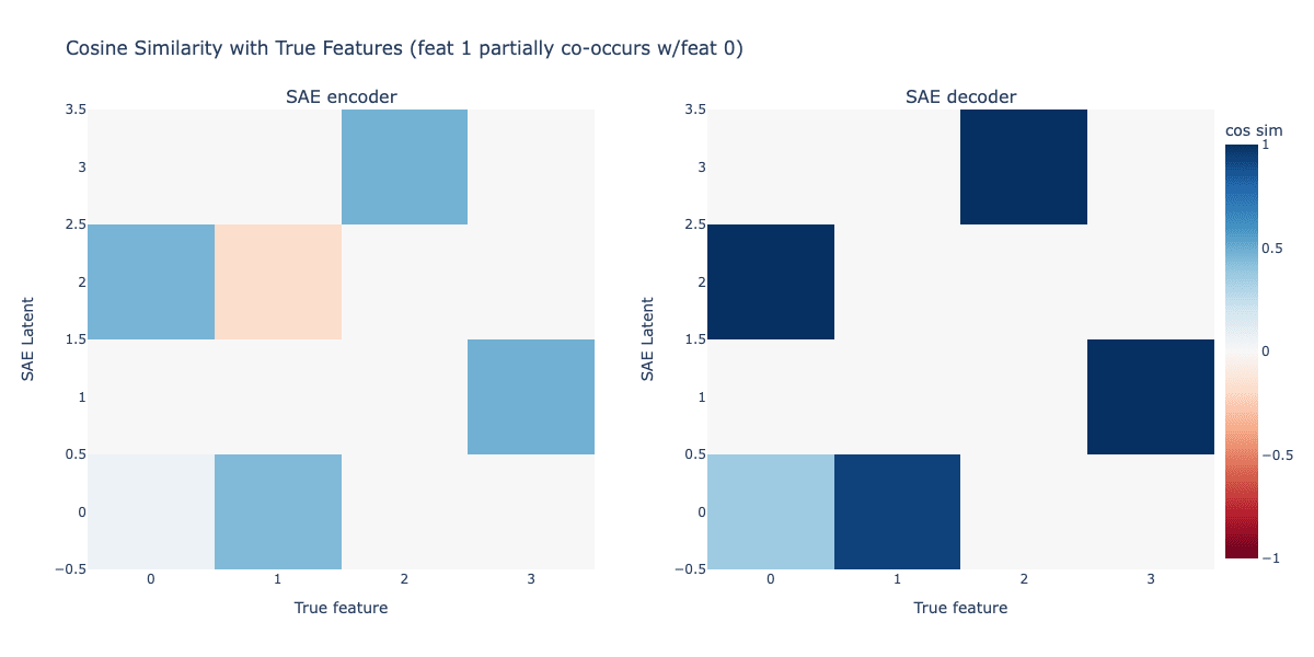
Next, we modify the firing pattern of feature 1 so it fires only if feature 0 also fires. However, we keep the overall firing rate of feature 1 the same as before, firing in 5% of activations. Features 2 and 3 remain independent.

Here, we see a crystal clear example of feature absorption. Latent 0 has learned a perfect representation of feature 0, but the encoder has a hole in it! Latent 0 fires if feature 0 is active but not feature 1! This is exactly the sort of gerrymandered feature firing pattern we saw in Gemma Scope SAEs for the starting letter task - the encoder has learned to stop the latent firing on specific cases where it looks like it should be firing. In addition, we see that latent 3, which tracks feature 1, has absorbed the feature 0 direction! This results in latent 3 representing a combination of feature 0 and feature 1. We see that the independently firing features 2 and 3 are untouched - the SAE still learns perfect representations of these features.
We can see this absorption in some sample firing patterns below:
| True features | SAE Latents | |||||||
|---|---|---|---|---|---|---|---|---|
| 0 | 1 | 2 | 3 | 0 | 1 | 2 | 3 | |
| Sample input 1 | 1.00 | 0 | 0 | 0 | 0.99 | 0 | 0 | 0 |
| Sample input 2 | 1.00 | 1.00 | 0 | 0 | 0 | 0 | 0 | 1.42 |
| Sample input 3 | 0 | 0 | 1.00 | 0 | 0 | 0 | 1.00 | 0 |
Notably, only one SAE latent fires when both feature 0 and feature 1 are active.
Magnitude variance causes partial absorption
We next adjust the scenario above so that there is some variance in the firing magnitude of feature 0. We allow the firing magnitude to vary with a standard deviation of 0.1. In real LLMs, we expect that features will have some slight differences in their activation magnitudes depending on the context, so this should be a realistic adjustment.
Here we still see the characteristic signs of feature absorption: the latent tracking feature 0 has a clear hole in it for feature 1, and the latent tracking feature 1 has absorbed the representation of feature 0. However, the absorption in the decoder is slightly less strong that it was previously. Investigating some sample firing patterns, we see the following:
| True features | SAE Latents | |||||||
|---|---|---|---|---|---|---|---|---|
| 0 | 1 | 2 | 3 | 0 | 1 | 2 | 3 | |
| Sample input 1 | 1.00 | 0 | 0 | 0 | 0 | 1.14 | 0 | 0 |
| Sample input 2 | 1.00 | 1.00 | 0 | 0 | 0 | 0.20 | 0 | 1.37 |
| Sample input 3 | 0.90 | 1.00 | 0 | 0 | 0 | 0.10 | 0 | 1.37 |
| Sample input 4 | 0.75 | 1.00 | 0 | 0 | 0 | 0 | 0 | 1.37 |
Here when feature 0 and feature 1 both fire with magnitude 1.0, we see the latent tracking feature 0 still activates, but very weakly. If the magnitude of feature 0 drops to 0.75, the feature turns off completely.
We call this phenomemon partial absorption. In partial absorption, there's co-occurrence between a dense and sparse feature, and the sparse feature absorbs the direction of the dense feature. However, the SAE latent tracking the dense feature still fires when both the dense and sparse feature are active, only very weakly. If the magnitude of the dense feature drops below some threshold, it stops firing entirely.
Why does partial absorption happen?
Feature absorption is an optimal strategy for minimizing the L1 loss and maximizing sparsity. However, when a SAE absorbs one latent into another, the absorbing latent loses the ability to modulate the magnitudes of the underlying features relative to each other. The SAE can address this by firing the latent tracking the dense feature as a "correction" to add back some of the dense feature direction into the reconstruction. Since the dense feature latent is firing weakly, it still has lower L1 loss than if the SAE fully separated out the features into their own latents.
Imperfect co-occurrence can still lead to absorption depending on L1 penalty
Next, let's test what will happen if feature 1 is more likely to fire if feature 0 is active, but can still fire without feature 0. We set up feature 1 to co-occur with feature 0 95% of the time, but 5% of the time it can fire on its own.
Here we see the telltale markers of feature absorption, but they are notably reduced in magnitude relative to the examples above.
| True features | SAE Latents | |||||||
|---|---|---|---|---|---|---|---|---|
| 0 | 1 | 2 | 3 | 0 | 1 | 2 | 3 | |
| Sample input 1 | 1.00 | 0 | 0 | 0 | 0 | 0 | 1.00 | 0 |
| Sample input 2 | 1.00 | 1.00 | 0 | 0 | 1.07 | 0 | 0.61 | 0 |
| Sample input 3 | 0 | 1.00 | 0 | 0 | 0.93 | 0 | 0 | 0 |
Despite the slight signs of absorption, we see the SAE latent tracking feature 0 still does fire when feature 1 and feature 0 are active together, although with reduced magnitude. This still isn't ideal as it means that the latents learned by the SAE don't fully match the true feature representations, but at least the latents all fire when they should! But will this still hold if we increase the L1 penalty on the SAE?
Next, we increase the L1 coefficent from 5e-3 to 2e-2 and train a new SAE.
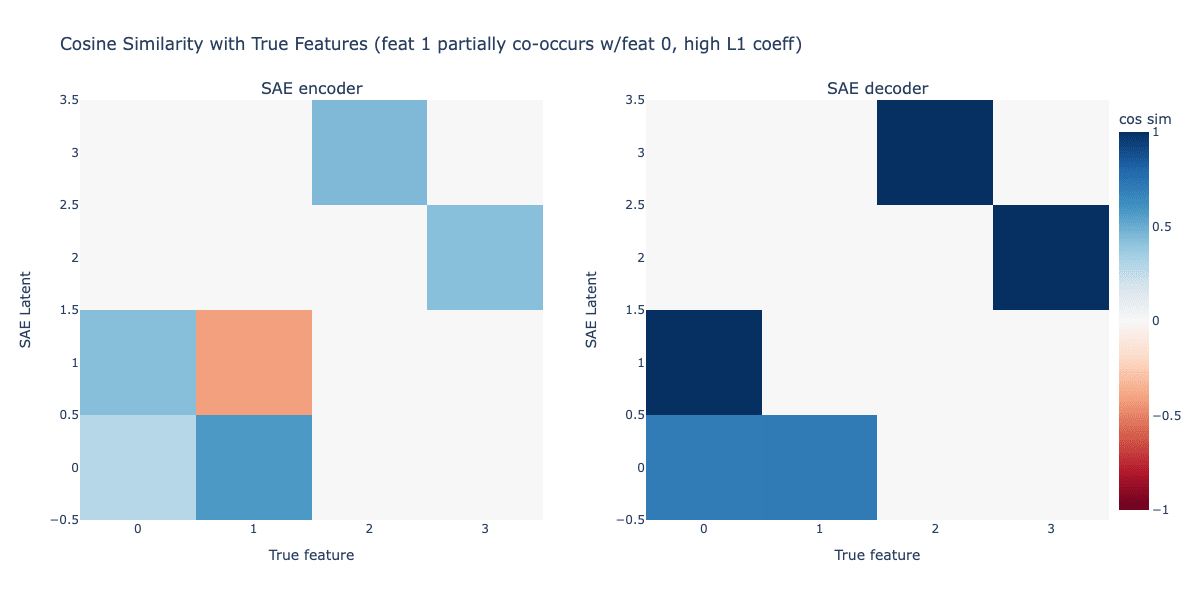
With this higher L1 coefficient, we see a much stronger feature absorption pattern in the encoder and decoder. Strangely, we also see the encoder for the latent tracking feature 1 encoding some of feature 0 - we don't have an explanation of why that happens with partial co-occurrence. Regardless, let's check the firing patterns for the SAE now:
| True features | SAE Latents | |||||||
|---|---|---|---|---|---|---|---|---|
| 0 | 1 | 2 | 3 | 0 | 1 | 2 | 3 | |
| Sample input 1 | 1.00 | 0 | 0 | 0 | 0 | 0.98 | 0 | 0 |
| Sample input 2 | 1.00 | 1.00 | 0 | 0 | 1.40 | 0 | 0 | 0 |
| Sample input 3 | 0 | 1.00 | 0 | 0 | 0.70 | 0 | 0 | 0 |
The firing patterns show feature absorption has occurred, where the latent tracking feature 0 fails to fire when both feature 0 and feature 1 are active. Here we see that the extent of the absorption increases as we increase our sparsity penalty. This makes sense as feature absorption is a sparsity-maximizing strategy for the SAE.
Tying the SAE encoder and decoder weights solves feature absorption
Looking at the patterns associated with absorption above, we always see a characteristic asymmetry between the SAE encoder and decoder. The SAE encoder creates a hole in the firing pattern of the dense co-occuring feature, but does not modify the decoder for that feature. Likewise, the absorbing feature encoder remains unchanged, but the decoder represents a combination of both co-occuring features. This points to a simple solution: what if we force the SAE encoder and decoder to share weights?
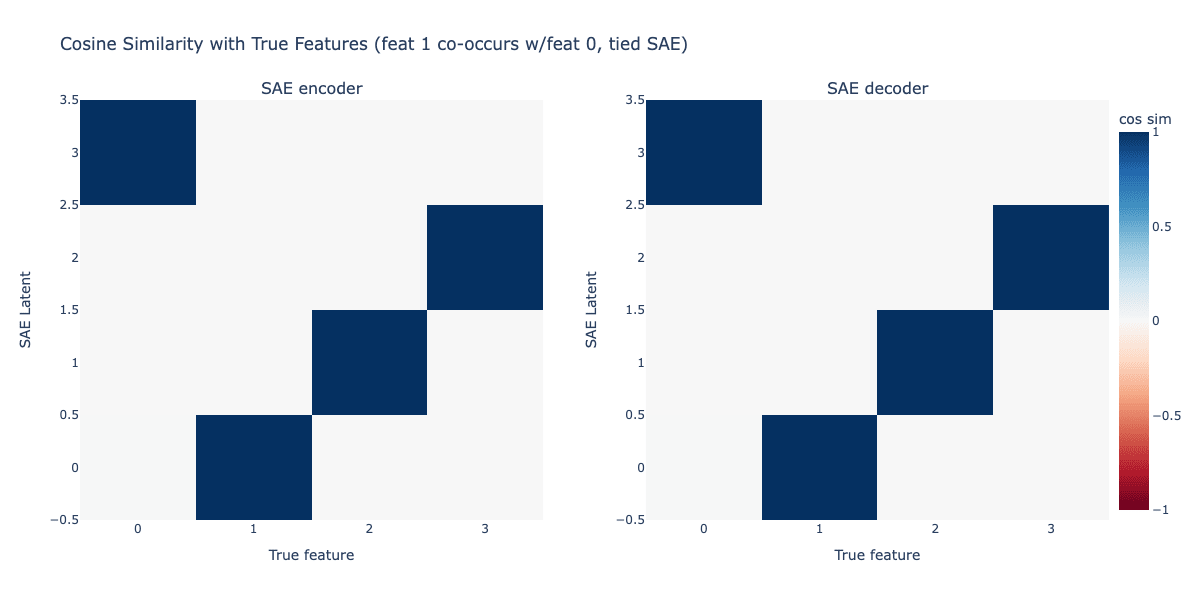
Amazingly, this simple fix seems to solve feature absorption! The SAE encoder and decoder learn the true feature representations! But this is a simple setup with no superposition; will this still work when we introduce more features and put them into superposition?
Absorption in superposition
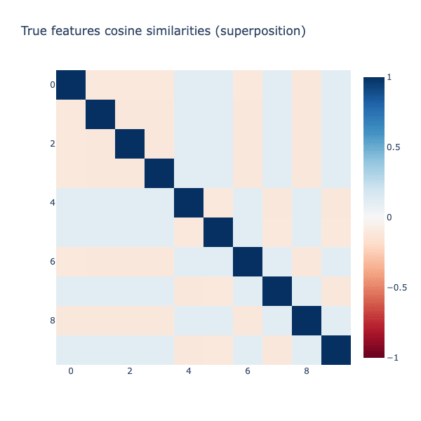
To induce superposition, we now use a toy model with 10 features, each with a 9 dimensional representation. We then optimize these representations to be as orthogonal as possible, but there is still necessarily going to be overlap between feature representations. Below we show the cosine similarities between all true features in this setup. Features have about ±10% cosine similarity with all other features. This is actually more intense superposition than we would expect in a real LLM, but should thus be a good test!
Next, we create our original feature absorption setup except with 10 features instead of 4. Feature 0 has a 25% firing probability. Features 1-9 all have a 5% firing probability. Feature 1 can only fire if feature 0 fires. All features fire with magnitude 1.0. We also increase the L1 penalty to 3e-2, as this seems necessary given the superposition.
First, we try using our original SAE setup to verify that absorption still happens in superposition.
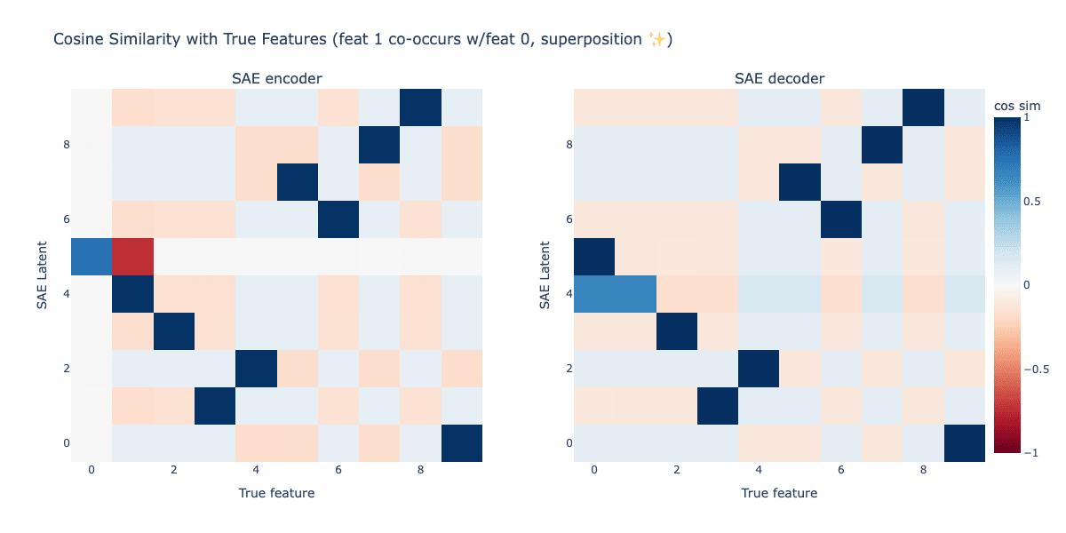
We still see the same characteristic absorption pattern between features 0 and 1. the encoder for the latent tracking feature 0 has a hole at feature 1, and the decoder for the latent tracking feature 1 represents a mix of feature 0 and 1 together. Interestingly, the encoder latent for feature 0 really emphasizes minimizing interference with features 2-9 in order to maximize the clarity of absorption! It's like the SAE is priorititizing absorption over everything else.
Tying the encoder and decoder weights still solves feature absorption in superposition.
Next, we try tying together the SAE encoder and decoder weights while keeping the same absorption setup as before.
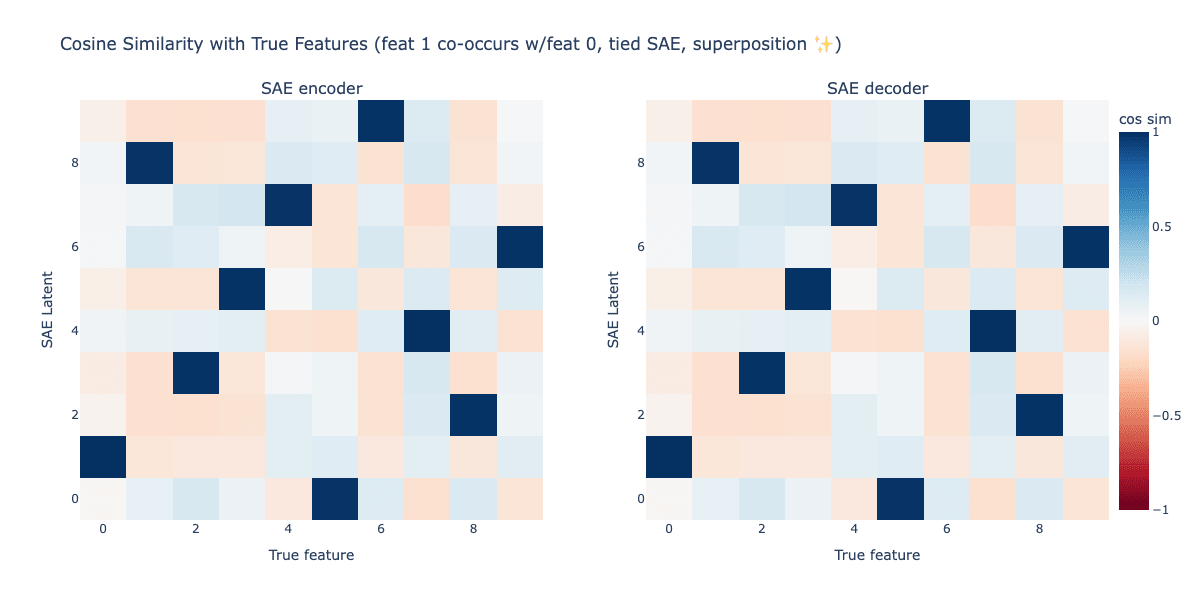
... And the SAE is still able to perfectly recover all feature representations, despite superposition! Hooray!
However this isn't without downside - the MSE loss is no longer 0 as it was before superposition.
Future work
While tying the SAE encoder and decoder weights seems to solve feature absorption in the toy examples here, we haven't yet tested this out on a non-toy SAE. It's also likely that tying together the encoder and decoder will result in higher MSE loss, but there may be ways of mitigating this by using a loss term that encourages the encoder and decoder to be as similar as possible while allowing slight asymmetries between them, or fine-tuning the encoder separately in a second run. We also have not tried out this tied encoder / decoder setup on the combo feature toy model [LW · GW]setup, so while this seems to fix absorption, it's possible this solution may not help combo latent issues.
Another promising direction may be to try deconstructing SAEs into denser components using Meta SAEs [AF · GW], and building the SAE out of these meta-latents. It's also likely there are more ways to solve absorption, such as adding an orthogonality loss [LW · GW] or other novel loss terms, or constructing the SAE in other novel ways.
Acknowledgements
Thank you to LASR Labs for making the original feature absorption work possible!
8 comments
Comments sorted by top scores.
comment by Michael Pearce (michael-pearce) · 2024-10-07T17:50:12.269Z · LW(p) · GW(p)
A hacky solution might be to look at the top activations using encoder directions AND decoder directions. We can think of the encoder as giving a "specific" meaning and the decoder a "broad" meaning, potentially overlapping other latents. Discrepancies between the two sets of top activations would indicate absorption.
Untied encoders give sparser activations by effectively removing activations that can be better attributed to other latents. So an encoder direction’s top activations can only be understood in the context of all the other latents.
Top activations using the decoder direction would be less sparse but give a fuller picture that is not dependent on what other latents are learned. The activations may be less monosemantic though, especially as you move towards weaker activations.
Replies from: chanind↑ comment by chanind · 2024-10-07T18:43:46.472Z · LW(p) · GW(p)
That's an interesting idea! That might help if training a new SAE with tied encoder/decoder (or some loss which encourages the same thing) isn't an option. It seems like with absorption you're still going to get mixes of of multiple features in the decoder, and a mix of the correct feature and the negative of excluded features in the encoder, which isn't ideal. Still, it's a good question whether it's possible to take a trained SAE with absorption and somehow identify the absorption and remove it or mitigate it rather than training from scratch. It would also be really interesting if we could find a way to detect absorption and use that as a way to quantify the underlying feature co-occurrences somehow.
I think you're correct that tying the encoder and decoder will mean that the SAE won't be as sparse. But then, maybe the underlying features we're trying to reconstruct are themselves not necessarily all sparse, so that could potentially be OK. E.g. things like "noun", "verb", "is alphanumeric", etc... are all things the model certainly knows, but would be dense if tracked in a SAE. The true test will be to try training some real tied SAEs and seeing how interpretable the results look like.
comment by Charlie Steiner · 2024-10-07T20:15:26.947Z · LW(p) · GW(p)
Amen. Untied weights are a weird hack. Problem is, they're a weird hack that, if you take it away, you have a lot less sparsity in your SAEs on real problems.
Now, to some extent you might want to say "well then you should accept that your view of model representations was wrong rather than trying to squeeze them onto a procrustean bed" but also also, the features found using untied weights are mostly interpretable and useful.
So another option might be to say "Both tied weights and untied weights are actually the wrong inference procedure for sparse features, and we need to go back to Bayesian methods or something."
Replies from: chanind↑ comment by chanind · 2024-10-08T10:42:45.195Z · LW(p) · GW(p)
I'm not as familiar with the history of SAEs - were tied weights used in the past, but then abandoned due to resulting in lower sparsity? If that sparsity is gained by creating feature absorption, then it's not a good thing since absorption does lead to higher sparsity but worse interpretability. I'm uncomfortable with the idea that higher sparsity is always better since the model might just have some underlying features its tracking that are dense, and IMO the goal should be to recover the model's "true" features, if such a thing can be said to exist, rather than maximizing sparsity which is just a proxy metric.
The thesis of this feature absorption work is that absorption causes latents that look interpretable but actually aren't. We initially found this initially by trying to evaluate the interpretability of Gemma Scope SAEs and found that latents which seemed to be tracking an interpretable feature have holes in their recall that didn't make sense. I'd be curious if tied weights were used in the past and if so, why they were abandoned. Regardless, it seems like the thing we need to do next for this work is to just try out variants of tied weights for real LLM SAEs and see if the results are more interpretable, regardless of the sparsity scores.
Replies from: kaden-uhlig↑ comment by K. Uhlig (kaden-uhlig) · 2024-10-08T14:44:06.728Z · LW(p) · GW(p)
Originally they were tied (because it makes intuitive sense), but I believe Anthropic was the first to suggest untying them, and found that this helped it differentiate similar features:
However, we find that in our trained models the learned encoder weights are not the transpose of the decoder weights and are cleverly offset to increase representational capacity. Specifically, we find that similar features which have closely related dictionary vectors have encoder weights that are offset so that they prevent crosstalk between the noisy feature inputs and confusion between the distinct features.
That post also includes a summary of Neel Nanda's replication of the experiments, and they provided an additional interpretation of this that I think is interesting.
Replies from: chanindOne question from this work is whether the encoder and decoder should be tied. I find that, empirically, the decoder and encoder weights for each feature are moderately different [AF · GW], with median cosine similiarty of only 0.5, which is empirical evidence they're doing different things and should not be tied. Conceptually, the encoder and decoder are doing different things: the encoder is detecting, finding the optimal direction to project onto to detect the feature, minimising interference with other similar features, while the decoder is trying to represent the feature, and tries to approximate the “true” feature direction regardless of any interference.
↑ comment by chanind · 2024-10-09T10:34:39.478Z · LW(p) · GW(p)
Thank you for sharing this! I clearly didn't read the original "Towards Monsemanticity" closely enough! It seems like the main argument is that when the weights are untied, the encoder and decoder learn different vectors, thus this is evidence that the encoder and decoder should be untied. But this is consistent with the feature absorption work - we see the encoder and decoder learning different things, but that's not because the SAE is learning better representations but instead because the SAE is finding degenerate solutions which increase sparsity.
Are there are any known patterns of feature firings where untying the encoder and decoder results in the SAE finding the correct or better representations, but where tying the encoder and decoder does not?
Replies from: TheMcDouglas↑ comment by CallumMcDougall (TheMcDouglas) · 2024-10-12T21:05:50.241Z · LW(p) · GW(p)
I don't know of specific examples, but this is the image I have in my head when thinking about why untied weights are more free than tied weights:
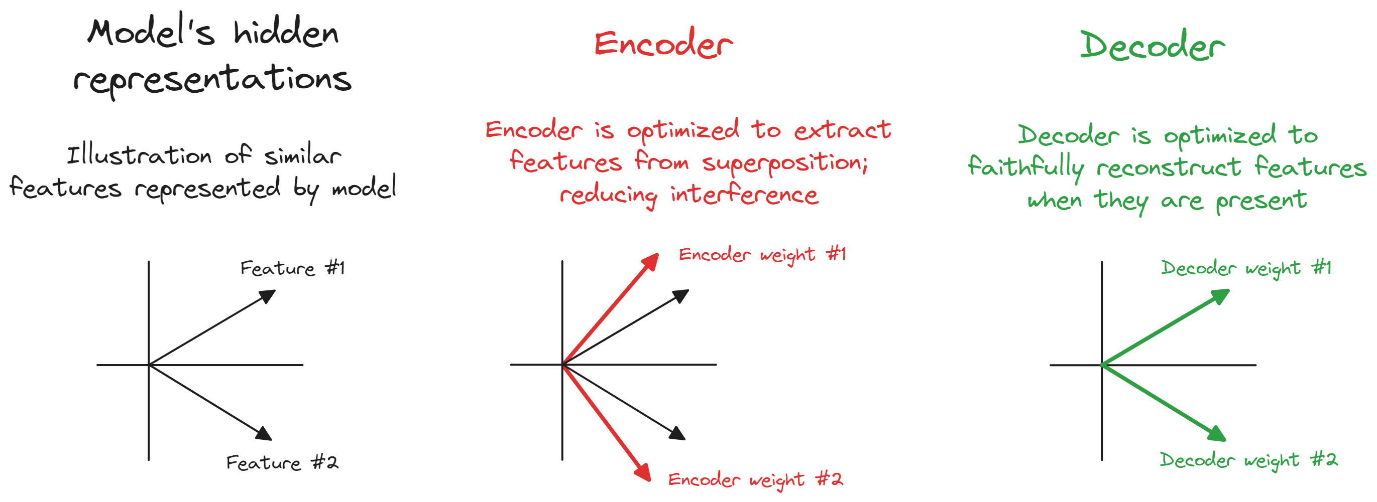
I think more generally this is why I think studying SAEs in the TMS setup can be a bit challenging, because there's often too much symmetry and not enough complexity for untied weights to be useful, meaning just forcing your weights to be tied can fix a lot of problems! (We include it in ARENA mostly for illustration of key concepts, not because it gets you many super informative results). But I'm keen for more work like this trying to understand feature absorption better in more tractible cases
Replies from: roger-d-1↑ comment by RogerDearnaley (roger-d-1) · 2024-11-20T21:42:29.947Z · LW(p) · GW(p)
I think an approach I'd try would be to keep the encoder and decoder weights untied (or possibly add a loss term to mildly encourage them to be similar), but then analyze the patterns between them (both for an individual feature and between pairs of features) for evidence of absorption. Absorption is annoying, but it's only really dangerous if you don't know it's happening and it causes you to think a feature is inactive when it's instead inobviously active via another feature it's been absorbed into. If you can catch that consistently, then it turns from concerning to merely inconvenient.
This is all closely related to the issue of compositional codes: absorption is just a code entry that's compositional in the absorbed instances but not in other instances. The current standard approach to solving that is meta SAEs, which presumably should also help identify absorption. It would be nice to have a cleaner and simpler process than that: than that I've been wondering if it would be possible to modify top-k or jump-RELU SAEs so that the loss function cost for activating more common dictionary entries is lower, in a way that would encourage representing compositional codes directly in the SAE as two-or-more more common activations rather than one rare one. Obviously you can't overdo making common entries cheap, otherwise your dictionary will just converge on a basis for the embedding space you're analyzing, all of which are active all the time — I suspect using something like a cost proportional to might work, where is the dimensionality of the underlying embedding space and is the frequency of the dictionary entry being activated.