Ambiguous out-of-distribution generalization on an algorithmic task

post by Wilson Wu (wilson-wu), Louis Jaburi (Ansatz) · 2025-02-13T18:24:36.160Z · LW · GW · 0 comments

Contents

  Introduction
    Setup
  Experiments
    Ambiguous grokking
      Grokking either group
      Grokking the intersect
      Grokking only one group
      No grokking
    Measuring complexity
      Complexity of the grokked solution
      Complexity over time
    Determination and differentiation
      Perturbation sensitivity
      Total variation
      Determination across distribution shift
      Training Jacobian
  Discussion
None
No comments

Introduction

It's now well known that simple neural network models often "grok" algorithmic tasks. That is, when trained for many epochs on a subset of the full input space, the model quickly attains perfect train accuracy and then, much later, near-perfect test accuracy. In the former phase, the model memorizes the training set; in the latter, it generalizes out-of-distribution to the test set.

In the algorithmic grokking literature, there is typically exactly one natural generalization from the training set to the test set. What if, however, the training set were instead under-specified in such a way that there were multiple possible generalizations? Would the model grok at all? If so, which of the generalizing solutions would it choose? If the model followed Occam's razor, it would choose the simplest solution -- but what does "simplest" mean here? We explore these questions for the task of computing a finite group operation.

Setup

This section assumes some basic familiarity with group theory and can be skipped. The point is just that each model is trained on the intersection of two datasets $G_1$ and $G_2$; the intersection of the two test sets always has size $\ge 50\%.$

In existing work on grokking finite group operations (e.g. Chughtai et al.), a one-hidden-layer MLP model with two inputs $f:R^G\times R^G\to R^G$ is trained on the operations of a finite group $G$. The model takes as input a pair of elements $x,y\in G$, encoded as one-hot vectors in $R^G$, and is expected to output logits maximized at the product $xy\in G.$ Thus, the input space is the set of all pairs $G^2$, and the model is evaluated on its accuracy over the entire test space: 

$$\text{acc}\left(f\right)=|G{|}^{-2}\sum _{x,y\in G}1\left\{\arg \underset{z\in G}{max}f\right(x,y{)}_z=xy\}.$$

Previous work finds that training on an iid subsample of 40% of the total input space (so the training set has $0.4|G{|}^2$ points) is enough to grok the full multiplication table for various choices of $G$. (The most well-studied choice is the symmetric group $G=S_5$.) In our setup, we leave everything the same except for the choice of training set. We now choose two groups $G_1$ and $G_2$ such that $|G_1|=|G_2|$. Thinking of the two groups as two operations ${\ast }_1$ and ${\ast }_2$ on the same underlying set of elements, our ambiguous training set is the set of all pairs of elements such that the two group operations agree:

$$X_{\text{train}}=\left\{\right(x,y):x{\ast }_{1}y=x{\ast }_{2}y\}.$$

Note then that $X_{\text{train}}$ can be completed to the full multiplication table for either $G_1$ or $G_2$. 

To ensure that there are enough elements in $X_{\text{train}}$ for grokking to be possible, we need to construct $G_1$ and $G_2$ with large overlap. One way is to set $G_1=H\times Z/2Z$ and $G_2=H{⋊}_{\phi }Z/2Z$ for some group $H$ and $\phi \in \text{Aut}\left(H\right)$. Then, by construction, whenever $k_1=0\in Z/2Z$,

$$(h_1,k_1){\ast }_1(h_2,k_2)=(h_1{h}_2,k_1{k}_2)=(h_1{\phi }^{k_1}{h}_2,k_1{k}_2)=(h_1,k_1){\ast }_2(h_2,k_2).$$

Thus, the overlap between $G_1$ and $G_2$ is at least 50%. (In fact, it is generally somewhat larger than 50%, owing to the fixed points of $\phi$.) All examples we discuss will be of this form.

Experiments

Ambiguous grokking

Grokking either group

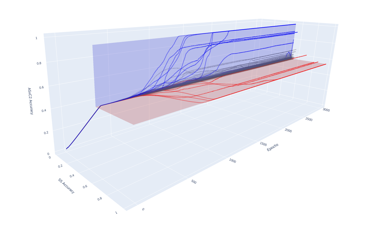
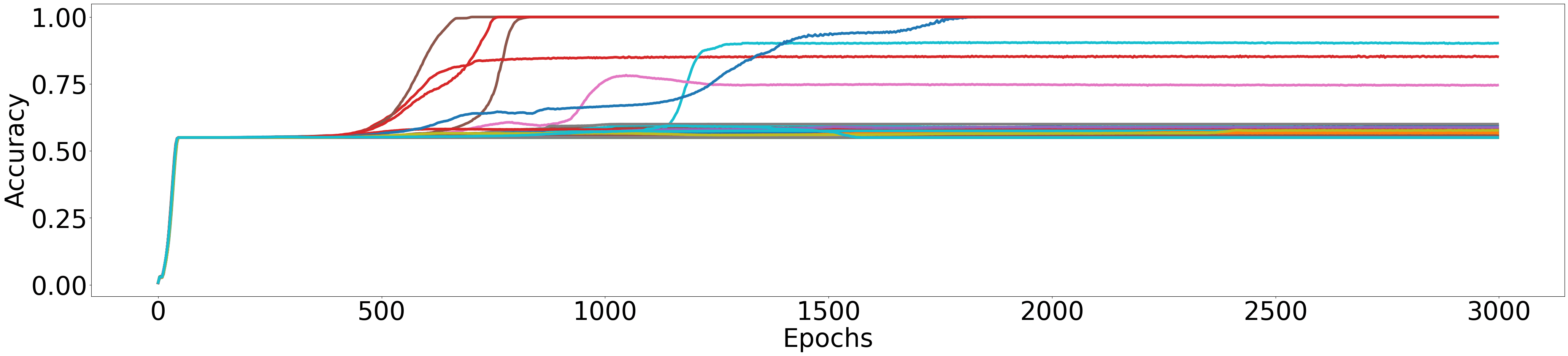
We run the training setup described above [LW(p) · GW(p)] with $G_1=S_5=A_5⋊Z/2Z$ and $G_2=A_5\times Z/2Z$. The intersection between the two groups' multiplication tables has size $7920/{120}^2=55\%$. We use this entire intersection as the training set and train 100 models with varying initialization seeds, all other hyperparameters held fixed. In this setup, the vast majority of models do not fully grok either solution (~90%), and instead just memorize $X_{\text{train}}$. However, we do find both models that grok $G_1$ (~4%) and $G_2$ (~6%).^[1]

Grokking the intersect

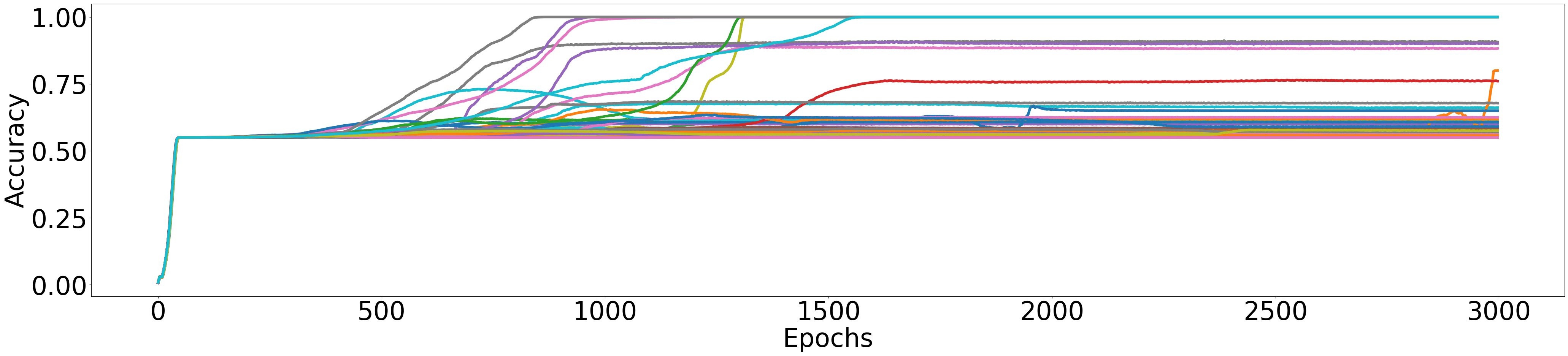
Although models often fail to grok either of the two groups, they always successfully grok the intersection: when we train models on an iid random 60% subset of the intersection (so 33% of the full input space), we find that they always attain full accuracy on the entire intersection and in some cases full accuracy on either $G_1$ or $G_2$.

Grokking only one group

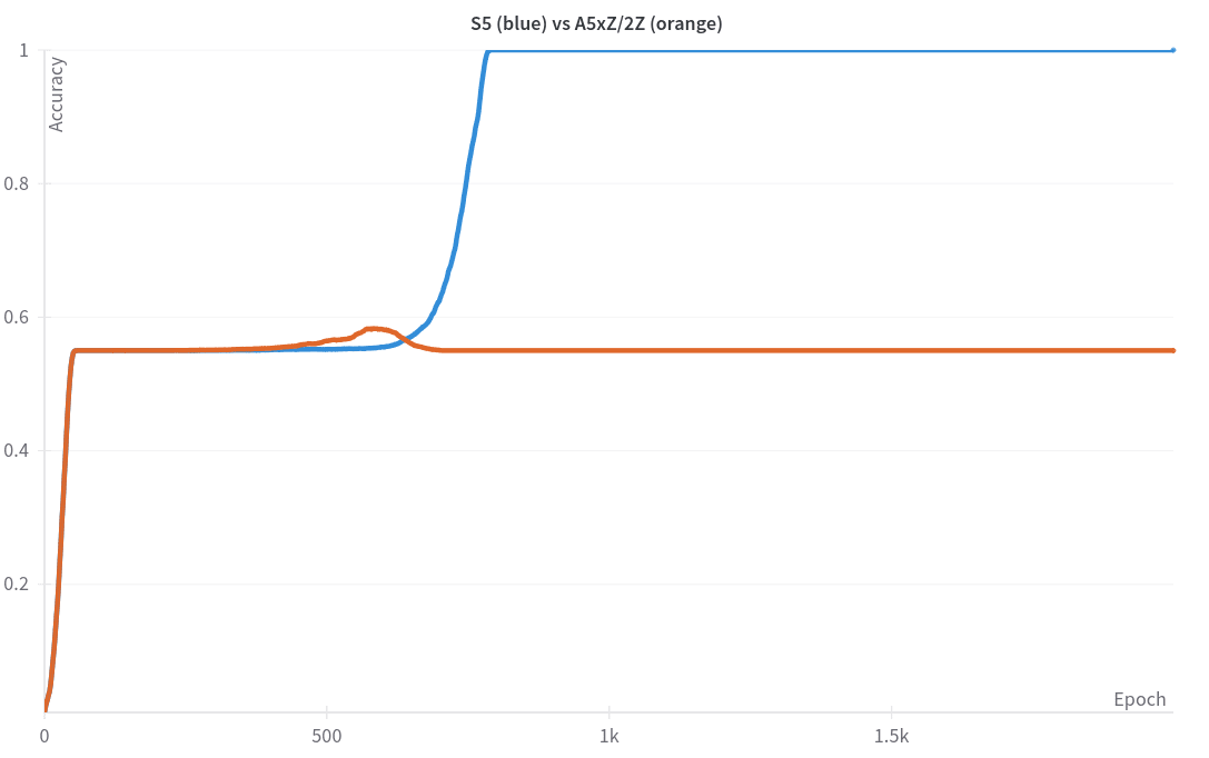
When we set $G_1=Z/48Z\times Z/2Z$ and $G_2=Z/48Z{⋊}_{\phi }Z/2Z$, where $\phi \in \text{Aut}\left(Z/48Z\right)$ maps $x\mapsto 25x$ (in this case, the intersection size is 75%), the model only groks $G_1$. Our intuition is that $G_1$, being commutative, is much simpler than $G_2$, which is not, and thus may be preferred by the model. This may just be a coincidence, however: we have not been able to find an intrinsic measure of group complexity such that models always prefer simpler groups. See more discussion below [LW · GW].

No grokking

When we set $G_1=Z/100Z$ and $G_1=Z/50Z\times Z/2Z$ (intersection size 51%) the model never groks either group. However, this example is a little unusual: the proportion of label classes in the intersect training set is non-uniform, and thus differs from the proportion over the entire input space (for either $G_1$ and $G_2$). We speculate that this class imbalance may be the reason for lack of grokking.

Measuring complexity

Complexity of the grokked solution

Intuitively, in cases where the model may grok either of two generalizing solutions, it should prefer the simpler of the two. There are two distinct things that we could mean by a solution implemented by a model being simple:

• The solution itself is simple, ignoring the model's implementation (i.e., treating the model as a black box). In our setting, this would correspond to the model learning simpler groups, for some intrinsic definition of the simplicity of a group. We had some hypotheses for what this group complexity measure could be, but were unable to empirically verify any of them.^[2]
• The model's implementation of the solution is simple (i.e., a white-box treatment). That is, the complexity measure is a function of the model's parameters, not just the group that it learns. There are various proposals in the literature for what the correct complexity measure in this sense could be. Two that we focus on are:
  • Circuit efficiency: Once a model has attained perfect training set accuracy, training cross-entropy loss can be made arbitrarily low by homogeneously scaling up the model weights. Assuming weight decay is non-zero (without which grokking is much more difficult to induce), this scaling introduces a natural trade-off between a solution's training loss and its ${\ell }_2$ weight norm. The circuit efficiency hypothesis is that the model chooses the solution that achieves the best training loss per unit weight norm.
  • Local learning coefficient (LLC): Roughly speaking, the LLC is a measure of basin broadness in a region around a given setting of model parameters. In the Bayesian setting, results from singular learning theory imply that, asymptotically, between two solutions with the same training loss, the model chooses that with lower LLC. Moreover, when the number of samples is finite, the model may even prefer models with lower LLC at the cost of higher training loss. (See the DSLT [? · GW] sequence.) The theory does not immediately transfer to models trained with SGD/Adam/etc., though there is empirical evidence that for such models the LLC still meaningfully measures the complexity of the model's internal structure (e.g. for modular arithmetic [LW · GW] and for language models).

To test whether LLC or some measure of circuit efficiency is able to predict which group the model groks, we train 10,000 models on the intersection of $G_1=S_4$ and $G_2=A_4\times Z/2Z$. In this setting, we again find that most models don't grok (93%). Among those that do grok there is a strong preference for $S_4$ (6.5%) over $A_4\times Z/2Z$ (0.5%). We then record the training loss, weight norm, and estimated LLC of all models at the end of training.

All three measures are somewhat predictive of what group is grokked, in a direction that aligns with our intuition that the model prefers simpler solutions. Models that grok $S_4$ (6.5%) tend to have lower training loss, weight norm, and LLC, and models that grok $A_4\times Z/2Z$ (0.5%) tend to have larger LLC and training loss, though still lower than what is typical for models that do not grok at all. However, we also find plenty of examples of models that do not grok either group yet still have low LLC and training loss. Possibly, these models are finding solutions that do not correspond to either of the two groups (or any group), yet still are "simple" in some appropriate sense.^[3]

Surprisingly, however, we observe that final training loss and weight norm are moderately correlated, and that final training loss and LLC are highly correlated.

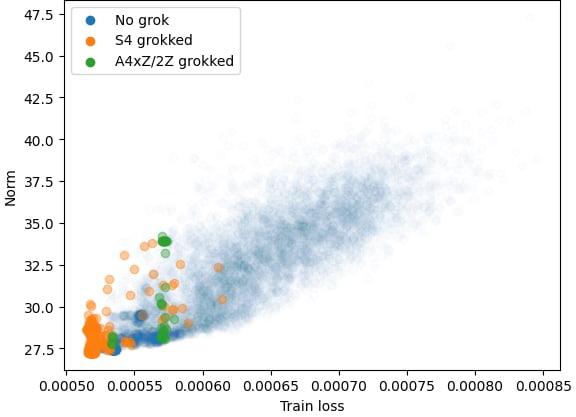
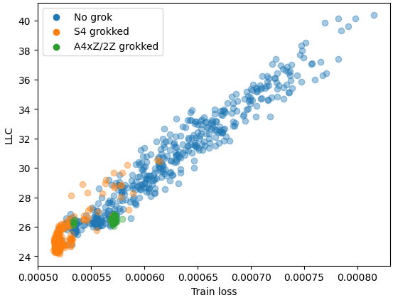
The correlation between training loss and LLC is especially unexpected to us, and we do not have a good explanation for its presence. Since (to our knowledge) this correlation has not been noted in other settings, we suspect that it is a quirk specific to 1-hidden layer MLPs trained on groups. In any case, while our results are suggestive that models prefer simpler solutions as measured by some combination of circuit efficiency and LLC, this correlation means that we cannot disentangle the two measures in the groups setting.

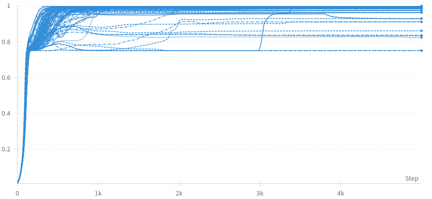
Complexity over time

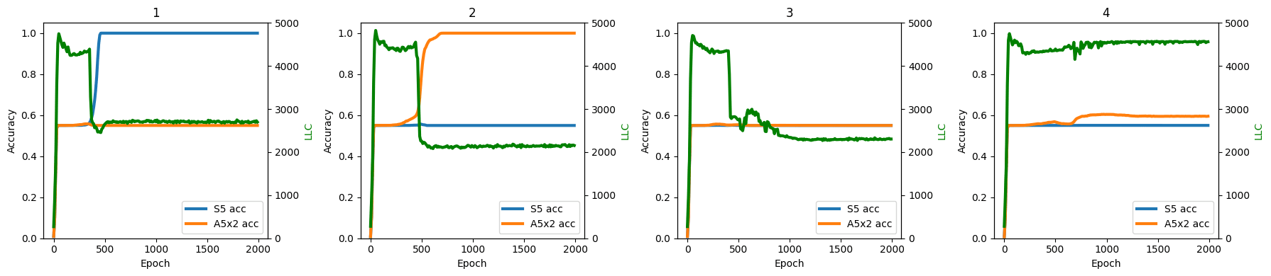
Besides checking model complexity at the end of training, we also measure it across training time. For $G_1=S_5$ and $G_2=A_5\times Z/2Z$, the LLC tracks grokking in the sense that, whenever the model groks either of the two groups, the LLC decreases sharply at the same time that the test accuracy rises. For models that do not grok either group, we observe both examples where the LLC stays large throughout training and examples where it falls. As aforementioned, we speculate that these cases correspond to the model learning some simple solution distinct from either of the two groups.

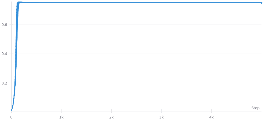
Are there any complexity measures that track grokking over time better than the LLC? We check those listed in Jiang et al. For simplicity, we measure these across checkpoints for a model trained on an iid subset of $S_5$ instead of an intersect set -- these models consistently grok. We notice that the LLC estimates in the iid case tend to be smoother over time than in the intersection experiments.

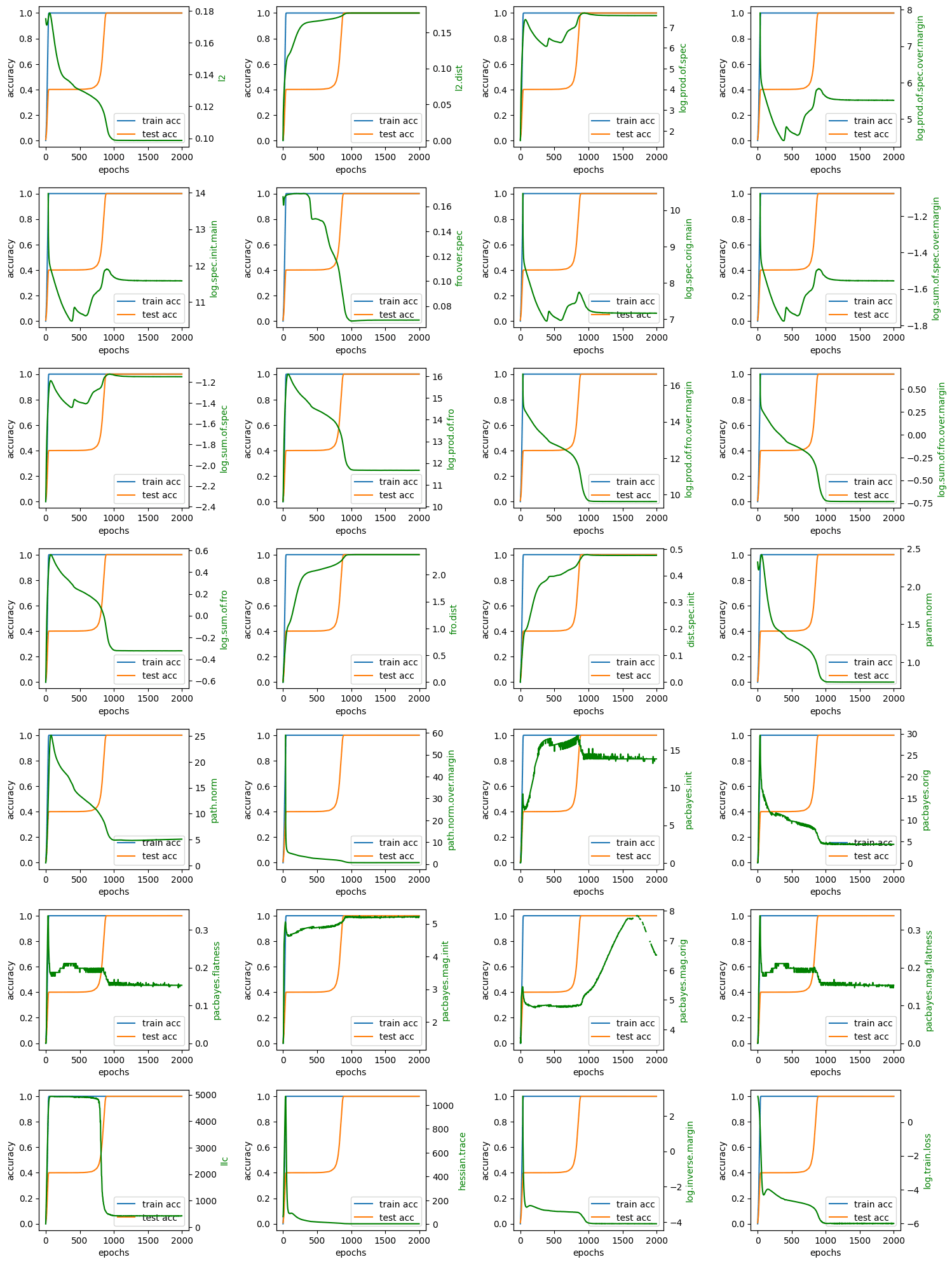
From these plots, it appears that LLC (bottom left) best tracks the generalization error, measured as the difference between train accuracy and test accuracy. Inverse margin and training loss (last two plots) also do well (perhaps this is related to the high correlation between training loss and LLC at the end of training, discussed above [? · GW]), but they are both large at the start of training, when generalization error is low because both training and test accuracy are low. The LLC is correctly low both at the beginning of training, before memorization, and at the end, after grokking.

Determination and differentiation

Perturbation sensitivity

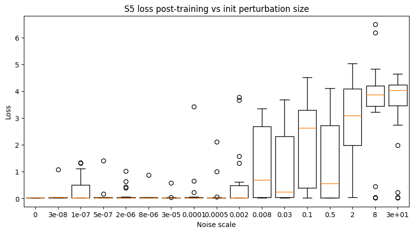
Somewhat separately from the previous investigations, one might wonder when the model "decides" which of the groups (if any) it will grok. In a literal sense, the answer is that the model's fate is determined at initialization, because in our experiments there is no stochasticity during training (we use full-batch gradient descent). However, this is not really a satisfying answer. Rather, when we say that the model has "decided" on a future solution, we should expect that, from the decision point onwards, its decision is robust: small perturbations in training should not be able to make the model "change its mind". 

Hence, to measure the point at which a model decides its fate, we make small Gaussian perturbations to the model weights at evenly spaced checkpoints throughout training. We then continue training anew from these perturbed weights. We find evidence that the model makes a decision not at initialization but still well before its choice is apparent in its test-set behavior.^[4]

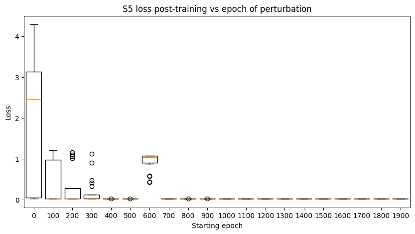
The example above is particularly interesting in that the model briefly veers towards $A_5\times Z/2Z$ around epoch 600, corresponding to a bump in perturbation sensitivity, before returning on its path towards $S_5$.^[5]

Total variation

For models trained on the intersection of two groups, we notice that those that grok either of the two groups tend to have more stable outputs late in training than those that grok neither. We quantify this by measuring total variation in logits over a fixed training interval:

$${\text{TV}}_{[i,j]}:=|G{|}^{-2}\sum _{n=i}^{j-1}\sum _{x,y\in G}1\left\{f_{{\theta }_n}\right(x,y)\ne f_{{\theta }_{n+1}}(x,y\left)\right\},$$

where ${\theta }_n$ are the model parameters at epoch $n$. For models trained on the intersection of $G_1=S_4$ and $G_2=A_4\times Z/2Z$ for 3000 epochs, we measure ${\text{TV}}_{[2500,3000]}$.

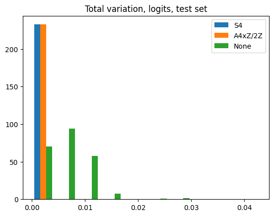
Models that grok either of $G_1,G_2$ always "lock in" their solutions -- the functions they compute no longer change after grokking. Those that grok neither often continue to oscillate in logit space even late in training.^[6] However, similarly to the case with the complexity measure experiments [LW · GW], there are many examples of models that grok neither and yet still have zero total variation, possibly corresponding to simple solutions distinct from both $G_1$ and $G_2$ that we are unaware of.

Note also that this is a purely test-set behavior. On the training set, all models have zero total variation by the end of training: once they attain perfect training accuracy, they no longer vary their training-set outputs.

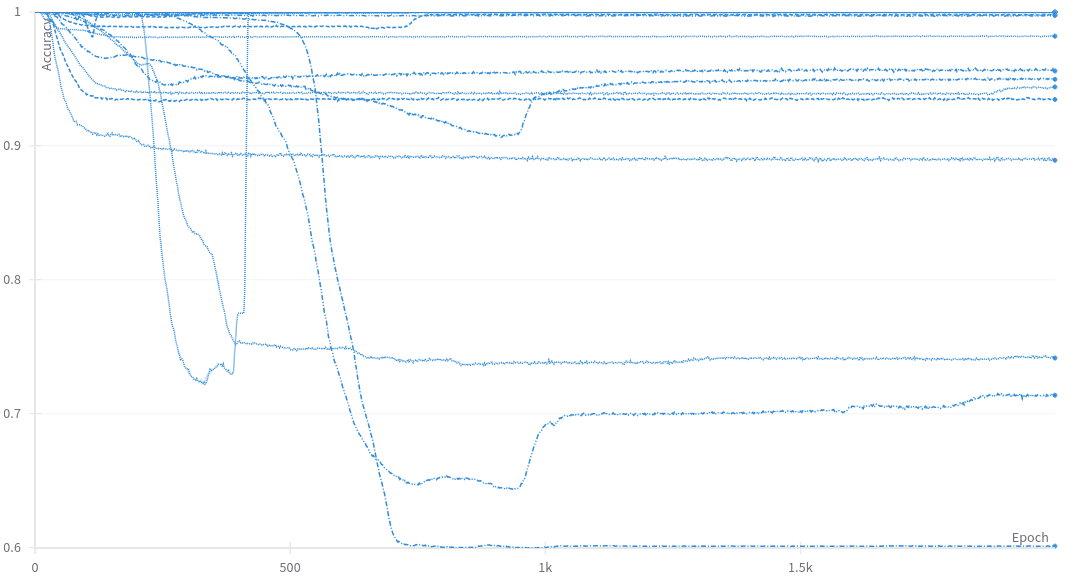
Determination across distribution shift

As seen above, the models that are trained on an intersection dataset and eventually grok have their fate stably determined relatively early in the training process. Is this stability a property of all possible parameter settings that implement the same solution? We investigate this question by first training models on iid data subsampled from $G_1=S_5$ so that the models consistently grok; we then "transplant" these models to the intersection of $G_1=S_5$ and $G_2=A_5\times Z/2Z$ and resume training. Perhaps surprisingly, many model instances (7%) partially ungrok $G_1$, while retaining perfect accuracy on the intersection. A few instances then proceed to regrok $G_1$, returning to perfect test accuracy later in training.^[7] Repeating the same experiment with the roles of $G_1$ and $G_2$ swapped results in the same behavior (8% ungrokked).

Training Jacobian

The training Jacobian (Belrose & Scherlis) is the Jacobian of the training map from initial model parameters to final model parameters.^[8] Thus, if the model has $m$ parameters, then the training map is of type $R^m\to R^m$ and the training Jacobian is a matrix $R^{m\times m}.$ In experiments with 25 epochs of training and without weight decay (hence no grokking), Belrose & Scherlis find that the training Jacobian preserves most directions in parameter space (corresponding to singular values $\approx 1$ and left singular vectors approximately equal to right singular vectors). The subspace approximately preserved by the training Jacobian is referred to as the bulk.

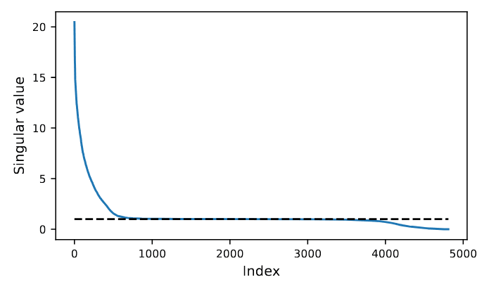
We compute the training Jacobian in our groups setting and observe that

• there is no bulk: extraneous directions in weight space are not preserved, but instead cleaned up by weight decay
• in the late stages of training, the training Jacobian blows up to infinity.

The results are similar across both models trained on group intersections and those trained on iid subsamples of one group.

Assuming the latter observation isn't an artifact of numerical instability, (which is entirely possible) we think it suggests that the limiting infinite-training map, mapping initial parameters to the fully converged final parameters, is discontinuous as a function $R^m\to R^m$. That is, arbitrarily small perturbations to the initial weights might cause non-negligible changes to the model's final weights.^[9] When the training set is iid, the different resulting model parameters all lead to the same model behaviors -- neural networks are non-identifiable. When the training set is under-determined, these changes in weight space may manifest as changes in model behavior.

As an aside, we note that this high sensitivity to model initialization seems to somewhat contradict (a sufficiently strong version of) the lottery ticket hypothesis. If there really existed a subnetwork at initialization that is significantly more amenable to training than the rest of the model, we'd expect its prominence to be at least somewhat robust to perturbations.

Discussion

We anticipate that ambiguous out-of-distribution generalization is a phenomenon that may arise not only in toy algorithmic tasks but also in more realistic settings. Indeed, recent work (Qin et al., Mészáros et al., Reizinger et al.) finds that the ability of language models to apply grammatical rules generalizes unstably out-of-distribution. Our concern is that ambiguous generalization may pose serious obstacles to the safety and alignment of LLM-based AI systems. Safety training for large language models is typically performed with datasets much smaller than those used for pre-training. Thus, safety training may be significantly more prone to under-specification in a manner leading to ambiguous generalization. Such under-specification may manifest in what is called deceptive alignment: the model appears to its designers to be well-aligned within the training environment, but in reality learns a solution that is harmful in deployment. Heuristic counting arguments (Hubinger [LW · GW], Carlsmith [LW · GW]) suggest that, in the presence of such ambiguity, true alignment may be vanishingly unlikely compared to deceptive alignment or scheming.

Our main motivation for studying models trained on the intersection of two groups was to 1) exhibit a crisp and concrete example of ambiguous generalization and 2) use the setting as a testbed for various hypotheses surrounding this phenomenon. Regarding 2), our hope was to relate some precise measure of a solution's complexity to the frequency with which it is learned, thus providing a quantitative version of the aforementioned counting arguments. While we were not able to fully attain this goal, we did find some evidence in favor of the local learning coefficient and circuit complexity. On the other hand, we were not able to disentangle these two measures in this toy setting, perhaps suggesting the need to move to other, more realistic experiments. Regardless, we continue to believe that ambiguous out-of-distribution generalization is an important, safety-relevant phenomenon that merits further study.

Acknowledgements: This work was mainly conducted during MATS 6.0 and 6.1. Many thanks to Jesse Hoogland, Daniel Filan, and Jacob Drori for helpful conversations. Wilson Wu was supported by an LTFF grant.

 

1. ^{^}

   Since in this experiment the sample size is small and grokking is somewhat rare, the proportion estimates should be treated as fairly low-confidence. In particular, we don't claim that the model prefers to grok $A_5\times Z/2Z$ over $S_5$. Our experiments [LW · GW] with $S_4$ and $A_4\times Z/2Z$ have a 100x larger sample size, and thus for those groups we are able to draw more confident conclusions about model preferences.

2. ^{^}

   One hypothesis we had was that the model would prefer the group with lower $c_s\left(G\right):={\sum }_{\rho \in \text{Irrep}\left(G\right)}\text{dim}(\rho {)}^s$ for some $s>2$. This quantity is larger for groups with larger irreps, and in particular is minimized for abelian groups. It also appears with $s=2.5$ in the expression for maximum margin computed in Theorem 9 of Morwani et al.'s paper. However, in the limited experiments we ran, this hypothesis seemed not to pan out.

3. ^{^}

   The functions computed by non-grokking models on the full input space are diverse and, in general, not simply combinations of $G_1$ and $G_2$.

4. ^{^}

   One might draw an analogy to cellular determination. "When a cell 'chooses' a particular fate, it is said to be determined, although it still 'looks' just like its undetermined neighbors. Determination implies a stable change -- the fate of determined cells does not change." (source)

5. ^{^}

   A speculative, likely incorrect cartoon picture: around epoch 300, the model is funneled into a slide in the loss landscape whose final destination is at $S_5$. Around epoch 600, there's a sharp bend in the slide (and/or it becomes narrower and/or shallower...). If the model takes the bend too quickly, it shoots over the edge and lands in $A_5\times Z/2Z.$

6. ^{^}

   We use a constant learning rate schedule. Likely this effect would not have been as apparent if we had instead used, say, cosine annealing.

7. ^{^}

   Performing some cursory mechanistic interpretability on these examples, we find that the original grokked parameters and the regrokked parameters generally differ, though they do tend to share many neurons in common (in the sense that the same neuron indices are supported in the same irreps). Since regrokking is a rare phenomenon that we only quickly spot-checked, we don't claim that this observation is representative.

8. ^{^}

   It follows immediately from the chain rule that, assuming the final model parameters are at a local minimum, the training Jacobian must lie in the null space of the loss Hessian at the final parameters. That is, the training Jacobian is only nontrivial if the model is singular.

9. ^{^}

   On the other hand, it is probably not too hard to show that any finite number of iterations of SGD, Adam, etc., is continuous. Only in the infinite training limit can discontinuities appear.

0 comments

Comments sorted by top scores.