Identifying Functionally Important Features with End-to-End Sparse Dictionary Learning
post by Dan Braun (dan-braun-1), Jordan Taylor (Nadroj), Nicholas Goldowsky-Dill (nicholas-goldowsky-dill), Lee Sharkey (Lee_Sharkey) · 2024-05-17T16:25:02.267Z · LW · GW · 20 commentsThis is a link post for https://arxiv.org/abs/2405.12241
Contents
  Introduction
  Key Results
  Acknowledgements
  Extras
None
20 comments
A short summary of the paper is presented below.
This work was produced by Apollo Research in collaboration with Jordan Taylor (MATS + University of Queensland) .
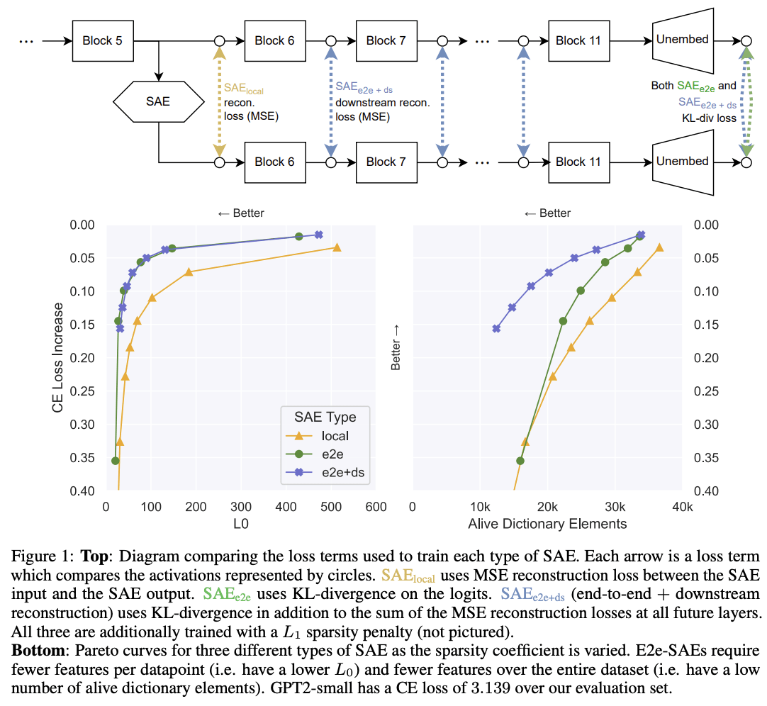
TL;DR: We propose end-to-end (e2e) sparse dictionary learning, a method for training SAEs that ensures the features learned are functionally important by minimizing the KL divergence between the output distributions of the original model and the model with SAE activations inserted. Compared to standard SAEs, e2e SAEs offer a Pareto improvement: They explain more network performance, require fewer total features, and require fewer simultaneously active features per datapoint, all with no cost to interpretability. We explore geometric and qualitative differences between e2e SAE features and standard SAE features.
Introduction
Current SAEs focus on the wrong goal: They are trained to minimize mean squared reconstruction error (MSE) of activations (in addition to minimizing their sparsity penalty). The issue is that the importance of a feature as measured by its effect on MSE may not strongly correlate with how important the feature is for explaining the network's performance.
This would not be a problem if the network's activations used a small, finite set of ground truth features -- the SAE would simply identify those features, and thus optimizing MSE would have led the SAE to learn the functionally important features. In practice, however, Bricken et al. observed the phenomenon of feature splitting, where increasing dictionary size while increasing sparsity allows SAEs to split a feature into multiple, more specific features, representing smaller and smaller portions of the dataset. In the limit of large dictionary size, it would be possible to represent each individual datapoint as its own dictionary element.
Since minimizing MSE does not explicitly prioritize learning features based on how important they are for explaining the network's performance, an SAE may waste much of its fixed capacity on learning less important features. This is perhaps responsible for the observation that, when measuring the causal effects of some features on network performance, a significant amount is mediated by the reconstruction residual errors (i.e. everything not explained by the SAE) and not mediated by SAE features (Marks et al.).
Given these issues, it is therefore natural to ask how we can identify the functionally important features used by the network. We say a feature is functional important if it is important for explaining the network's behavior on the training distribution. If we prioritize learning functionally important features, we should be able to maintain strong performance with fewer features used by the SAE per datapoint as well as fewer overall features.
To optimize SAEs for these properties, we introduce a new training method. We still train SAEs using a sparsity penalty on the feature activations (to reduce the number of features used on each datapoint), but we no longer optimize activation reconstruction. Instead, we replace the original activations with the SAE output and optimize the KL divergence between the original output logits and the output logits when passing the SAE output through the rest of the network, thus training the SAE end-to-end (e2e).
One risk with this method is that it may be possible for the outputs of SAE_e2e to take a different computational pathway through subsequent layers of the network (compared with the original activations) while nevertheless producing a similar output distribution. For example, it might learn a new feature that exploits a particular transformation in a downstream layer that is unused by the regular network or that is used for other purposes. To reduce this likelihood, we also add terms to the loss for the reconstruction error between the original model and the model with the SAE at downstream layers in the network.
It's reasonable to ask whether our approach runs afoul of Goodhart's law ("When a measure becomes a target, it ceases to be a good measure") We contend that mechanistic interpretability should prefer explanations of networks (and the components of those explanations, such as features) that explain more network performance over other explanations. Therefore, optimizing directly for quantitative proxies of performance explained (such as CE loss difference, KL divergence, and downstream reconstruction error) is preferred.
Key Results
We train each SAE type on language models (GPT2-small and Tinystories-1M), and present three key findings (Figure 1):
- For the same level of performance explained, SAE_local requires activating more than twice as many features per datapoint compared to SAE_e2e+downstream and SAE_e2e.
- SAE_e2e+downstream performs equally well as SAE_e2e in terms of the number of features activated per datapoint, yet its activations take pathways through the network that are much more similar to SAE_local.
- SAE_local requires more features in total over the dataset to explain the same amount of network performance compared with SAE_e2e and SAE_e2e+ds.
Moreover, our automated interpretability and qualitative analyses reveal that SAE_e2e+ds features are at least as interpretable as SAE_local features, demonstrating that the improvements in efficiency do not come at the cost of interpretability. These gains nevertheless come at the cost of longer wall-clock time to train (see article for further details).
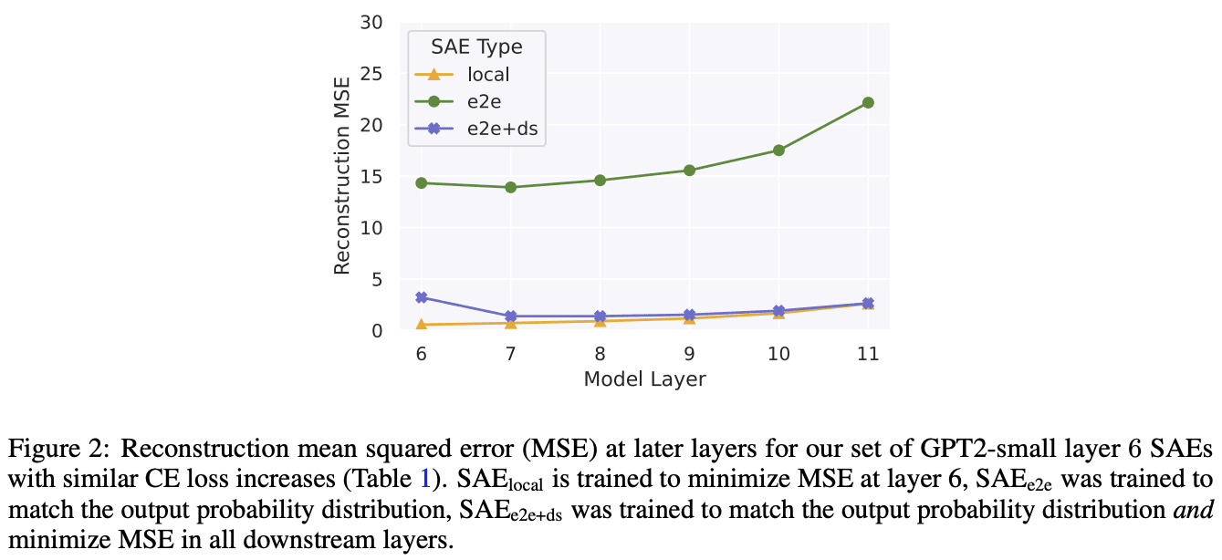
When comparing the reconstruction errors at each downstream layer after the SAE is inserted (Figure 2 below), we find that, even though SAE_e2es explain more performance per feature than SAE_locals, they have much worse reconstruction error of the original activations at each subsequent layer. This indicates that the activations following the insertion of SAE_e2e take a different path through the network than in the original model, and therefore potentially permit the model to achieve its performance using different computations from the original model. This possibility motivated the training of SAE_e2e+ds, which we see has extremely similar reconstruction errors compared to SAE_local. SAE_e2e+ds therefore has the desirable properties of both learning features that explain approximately as much network performance as SAE_e2e (Figure 1) while having reconstruction errors that are much closer to SAE_local.
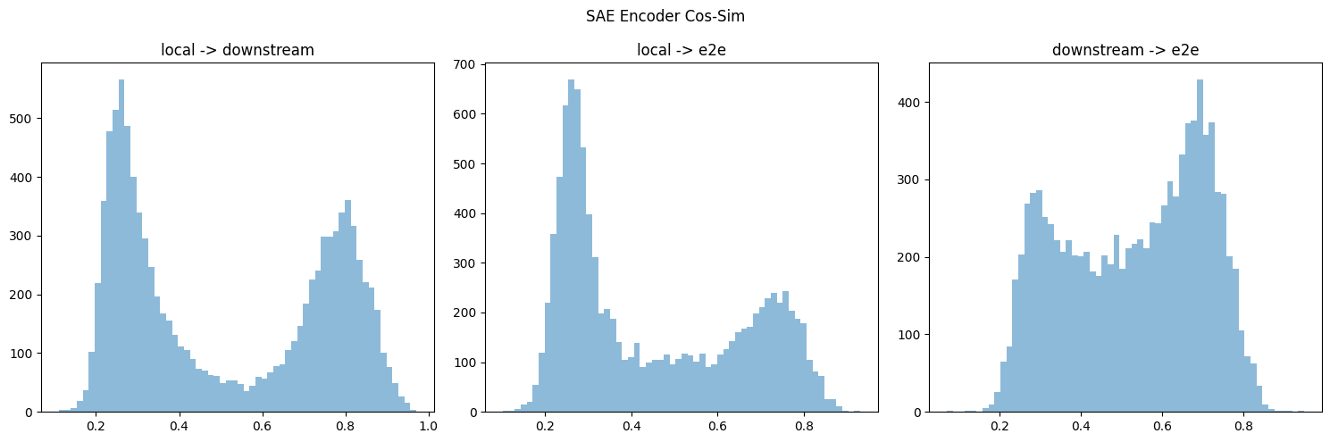
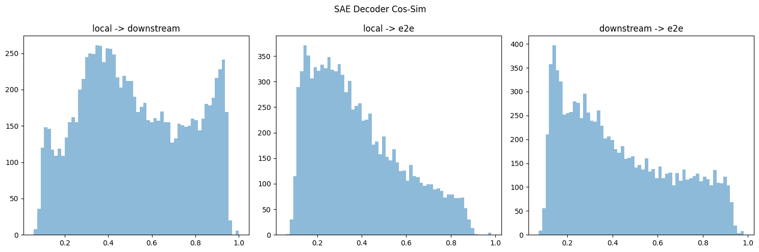
We measure the cosine similarities between each SAE dictionary feature and next-closest feature in the same dictionary. While this does not account for potential semantic differences between directions with high cosine similarities, it serves as a useful proxy for feature splitting, since split features tend to be highly similar directions. We find that SAE_local has features that are more tightly clustered, suggesting higher feature splitting (Figure 3 below). Compared to SAE_e2e+ds the mean cosine similarity is 0.04 higher (bootstrapped 95% CI [0.037-0.043]); compared to SAE_e2e the difference is 0.166 (95% CI [0.163-0.168]). We measure this for all runs in our Pareto frontiers in Appendix A.7 (Figure 7), and find that this difference is not explained by SAE_local having more alive dictionary elements than e2e SAEs.
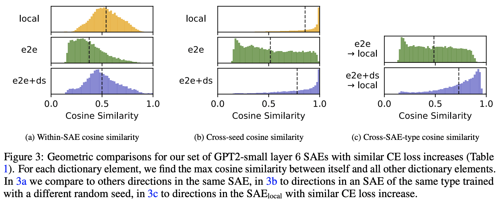
In the paper, we also explore some qualitative differences between SAE_local and SAE_e2e+ds.
Acknowledgements
Johnny Lin and Joseph Bloom for supporting our SAEs on https://www.neuronpedia.org/gpt2sm-apollojt and Johnny Lin for providing tooling for automated interpretability, which made the qualitative analysis much easier. Lucius Bushnaq, Stefan Heimersheim and Jake Mendel for helpful discussions throughout. Jake Mendel for many of the ideas related to the geometric analysis. Tom McGrath, Bilal Chughtai, Stefan Heimersheim, Lucius Bushnaq, and Marius Hobbhahn for comments on earlier drafts. Center for AI Safety for providing much of the compute used in the experiments.
Extras
- Library for training e2e (and vanilla) SAEs and reproducing our analysis (https://github.com/ApolloResearch/e2e_sae). All SAEs in the article can be loaded using this library, and we also provide raw SAE weights for many of our runs at https://huggingface. co/apollo-research/e2e-saes-gpt2.
- Weights and Biases report that links to training metrics for all runs https://api.wandb.ai/links/sparsify/evnqx8t6
- Neuronpedia page (h/t @Johnny Lin [LW · GW] @Joseph Bloom [LW · GW]) for interactively exploring many of the SAEs presented in the article (https://www.neuronpedia.org/gpt2sm-apollojt)
20 comments
Comments sorted by top scores.
comment by Logan Riggs (elriggs) · 2024-06-18T21:58:57.168Z · LW(p) · GW(p)
The e2e having different feature directions across seeds was quite the bummer, but then I thought "are the encoder directions different though?"
Intuitively the encoder directions affect which datapoints each feature activates on, and the decoder is the causal downstream effect. For e2e, we would expect widely different decoder directions because there are many free parameters (from some other work that showed SVD of gradients had many zero singular values, meaning moving in most directions don't effect the downstream loss), but not necessarily encoder directions.
If the encoder directions are similar across seeds, I'd trust them to inform relevant features for the model output (in cases where we don't care about connections w/ downstream layers).
However, I was not able to find the SAEs for various seeds.
Trying to replicate Cos-sim Plots
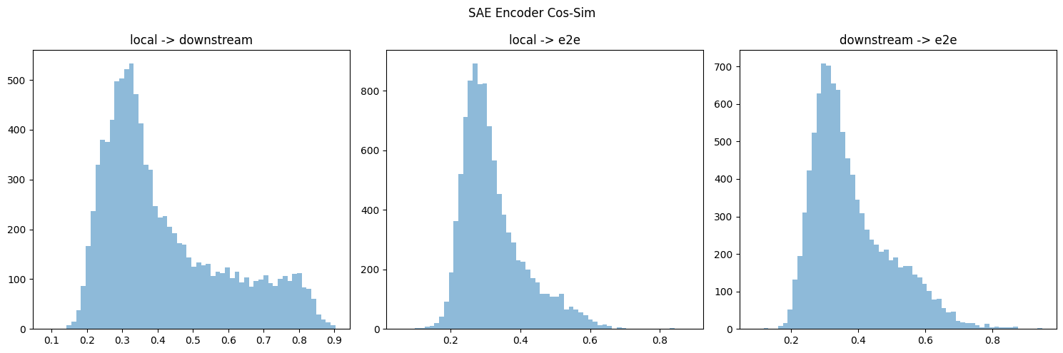
I downloaded the similar CE at layer 6 for all three types of SAEs & took their cos-sim (last column in figure 3).
I think your cos-sim metric gives different results if you take the max over the first or 2nd dimension (or equivalently swapped the order of decoders multiplied by each other). If so, I think this is because you might double-count or something? Regardless, I ended up doing some hungarian algorithm to take the overall max (but don't double-count), but it's on cpu, so I only did the first 10k/40k features. Below is results for both encoder & decoder, which do replicate the directional results.
Nonzero Features
Additionally I thought that some results were from counting nonzero features, which, for the encoder is some high-cos-sim features, and decoder is the low-cos-sim features weirdly enough.
Would appreciate if y'all upload any repeated seeds!
My code is temporarily hosted (for a few weeks maybe?) here.
Replies from: dan-braun-1↑ comment by Dan Braun (dan-braun-1) · 2024-06-19T08:52:15.534Z · LW(p) · GW(p)
Every SAE in the paper is hosted on wandb, only some are hosted on huggingface, so I suggest loading them from wandb for now. We’ll upload more to huggingface if several people prefer that. Info for downloading from wandb can be found in the repo, the easiest way is probably:
# pip install e2e_sae
# Save your wandb api key in .env
from e2e_sae import SAETransformer
model = SAETransformer.from_wandb("sparsify/gpt2/d8vgjnyc")
sae = list(model.saes.values())[0] # Assumes only 1 sae in model, true for all saes in paper
encoder = sae.encoder[0]
dict_elements = sae.dict_elements  # Returns the normalized decoder elements
The wandb ids for different seeds can be found in the geometric analysis script here. That script, along with plot_performance.py, is a good place to see which wandb ids were used for each plot in the paper, as well as the exact code used to produce the plots in the paper (including the cosine sim plots you replicated above).
If you want to avoid the e2e_sae dependency, you can find the raw sae weights in the samples_400000.pt file in the respective wandb run. Just make sure to normalize the decoder weights after downloading (note that this was done before uploading to huggingface so people could load the SAEs into e.g. SAELens without having to worry about it).
If so, I think this is because you might double-count or something?
We do double count in the sense that, if, when comparing the similarity between A and B, element A_i has max cosine sim with B_j, we don't remove B_j from being in the max cosine sim for other elements in A. It's not obvious (to me at least) that we shouldn't do this when summarising dictionary similarity in a single metric, though I agree there is a tonne of useful geometric comparison that isn't covered by our single number. Really glad you're digging deeper into this. I do think there is lots that can be learned here.
Btw it's not intuitive to me that the encoder directions might be similar even though the decoder directions are not. Curious if you could share your intuitions here.
Replies from: elriggs, elriggs↑ comment by Logan Riggs (elriggs) · 2024-08-22T17:22:14.624Z · LW(p) · GW(p)
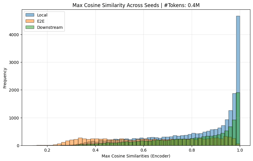
I finally checked!
Here is the Jaccard similarity (ie similarity of input-token activations) across seeds
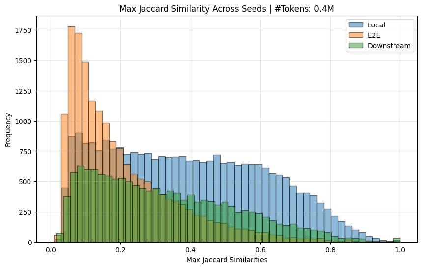
The e2e ones do indeed have a much lower jaccard sim (there normally is a spike at 1.0, but this is removed when you remove features that only activate <10 times).
I also (mostly) replicated the decoder similarity chart:
And calculated the encoder sim:
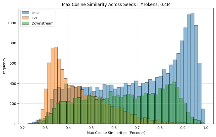
[I, again, needed to remove dead features (< 10 activations) to get the graphs here.]
So yes, I believe the original paper's claim that e2e features learn quite different features across seeds is substantiated.
↑ comment by Logan Riggs (elriggs) · 2024-06-19T15:40:43.942Z · LW(p) · GW(p)
Thanks so much! All the links and info will save me time:)
Regarding cos-sim, after thinking a bit, I think it's more sinister. For cross-cos-sim comparison, you get different results if you take the max over the 0th or 1st dimension (equivalent to doing cos(local, e2e) vs cos(e2e, local). As an example, you could have 2 features each, 3 point in the same direction and 1 points opposte. Making up numbers:
feature-directions(1D) = [ [1],[1]] & [[1],[-1]]
cos-sim = [[1, 1], [-1, -1]]
For more intuition, suppose 4 local features surround 1 e2e feature (and the other features are pointed elsewhere). Then the 4 local features will all have high max-cos sim but the e2e only has 1. So it's not just double-counting, but quadruple counting. You could see for yourself if you swap your dim=1 to 0 in your code.
But my original comment showed your results are still directionally correct when doing [global max w/ replacement] (if I coded it correctly).
Btw it's not intuitive to me that the encoder directions might be similar even though the decoder directions are not. Curious if you could share your intuitions here.
The decoder directions have degrees of freedom, but the encoder directions...might have similar degrees of freedom and I'm wrong, lol. BUT! they might be functionally equivalent, so they activate on similar datapoints across seeds. That is more laborious to check though, waaaah.
I can check both (encoder directions first) because previous literature is really only on the SVD of gradient (ie the output), but an SAE might be more constrained when separating out inputs into sparse features. Thanks for prompting for my intuition!
comment by Matthew Khoriaty (matthew-khoriaty) · 2025-01-14T03:36:48.573Z · LW(p) · GW(p)
Hi, I'm undertaking a research project and I think that an end2end SAE with automated explanations would be a lot of help.
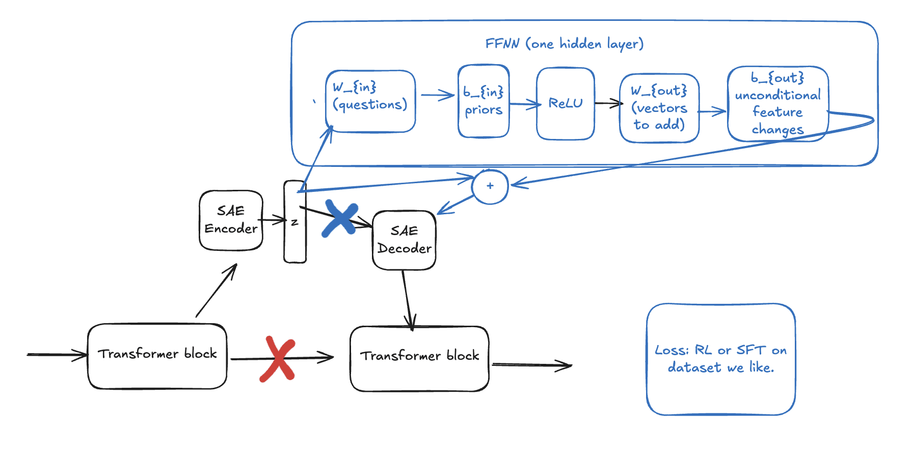
The project is a a parameter-efficient fine-tuning method that may be very interpretable, allowing researchers to know what the model learned during fine-tuning:
Start by acquiring a model with end-to-end SAEs throughout. Insert a 1 hidden layer FFNN (with a skip connection) after a SAE latent vector and pass the output to the rest of the model. Since SAE latents are interpretable, the rows in the first FFNN matrix will be interpretable as questions about the latent, and the columns of the second FFNN matrix will be interpretable as question-conditional edits to the residual latent vector as in https://www.alignmentforum.org/posts/iGuwZTHWb6DFY3sKB/fact-finding-attempting-to-reverse-engineer-factual-recall [AF · GW]
I would expect end2end SAEs to work better than local SAEs because as you found, local SAEs do not return decodings with the same behaviors as well as end2end SAEs.
If you could share your dict[SAE latent, description] for
e2e-saes-gpt , I would appreciate it so much. If you cannot, I'll use a local SAE instead for which I can find descriptions of the latents, though I expect it would not work as well.
Also, you might like to hear that some of your links are dead:
https://www.neuronpedia.org/gpt2sm-apollojt results in:
Error: Minified React error #185; visit https://react.dev/errors/185 for the full message or use the non-minified dev environment for full errors and additional helpful warnings.
Back to Home
https://huggingface.%20co/apollo-research/e2e-saes-gpt2 cannot be reached.
Replies from: hijohnnylin, dan-braun-1↑ comment by Johnny Lin (hijohnnylin) · 2025-01-15T20:14:17.153Z · LW(p) · GW(p)
apologies for the issue with the neuronpedia link. it's now been resolved.
↑ comment by Dan Braun (dan-braun-1) · 2025-01-14T09:18:04.028Z · LW(p) · GW(p)
Hey Matthew. We only did autointerp for 200 randomly sampled latents in each dict, rather than the full 60 × 768 = 46080 latents (although half of these die). So our results there wouldn't be of much help for your project unfortunately.
Thanks a lot for letting us know about the dead links. Though note you have a "%20" in the second one which shouldn't be there. It works fine without it.
Replies from: matthew-khoriaty↑ comment by Matthew Khoriaty (matthew-khoriaty) · 2025-01-14T17:02:03.064Z · LW(p) · GW(p)
Thank you, Dan.
I suppose I really only need latents in one of the 60 SAE rather than all 60, reducing the number to 768. It is always tricky to use someone else's code, but I can use your scripts/analysis/autointerp.py run_autointerp to label what I need. Could you give me an idea for how much compute that would take?
I was hoping to get your feedback on my project idea.
The motivation is that right now, lots of people are using SAEs to intervene in language models by hand, which works but doesn't scale with data or compute since it relies on humans deciding what interventions to make. It would be great to have trainable SAE interventions. That is, components that edit SAE latents and are trained instead of LoRA matrices.
The benefit over LoRA would be that if the added component is simple, such as z2 = z + FFNN(z), where the FFNN has only one hidden layer, then it would be possible to interpret the FFNN and explain what the model learned during fine-tuning.
I've included a diagram below. The X'es represent connections that are disconnected.
↑ comment by Dan Braun (dan-braun-1) · 2025-01-14T17:47:56.858Z · LW(p) · GW(p)
heh, unfortunately a single SAE is 768 * 60. The residual stream in GPT2 is 768 dims and SAEs are big. You probably want to test this out on smaller models.
I can't recall the compute costs for that script, sorry. A couple of things to note:
- For a single SAE you will need to run it on ~25k latents (46k minus the dead ones) instead of the 200 we did.
- You will only need to produce explanations for activations, and won't have to do the second step of asking the model to produce activations given the explanations.
It's a fun idea. Though a serious issue is that your external LoRA weights are going to be very large because their input and output will need to be the same size as your SAE dictionary, which could be 10-100x (or more, nobody knows) the residual stream size. So this could be a very expensive setup to finetune.
Replies from: matthew-khoriaty↑ comment by Matthew Khoriaty (matthew-khoriaty) · 2025-01-15T05:02:19.699Z · LW(p) · GW(p)
Thank you again.
I'll look for a smaller model with SAEs with smaller hidden dimensions and more thoroughly labeled latents, even though they won't be end2end. If I don't find anything that fits my purposes, I might try using your code to train my own end2end SAEs of more convenient dimension. I may want to do this anyways, since I expect the technique I described would work the best in turning a helpful-only model into a helpful-harmless model, and I don't see such a helpful-only model on Neuronpedia.
If the FFNN has a hidden dimension of 16, then it would have around 1.5 million parameters, which doesn't sound too bad, and 16 might be enough to find something interesting.
Low-rank factorization might help with the parameter counts.
Overall, there are lots of things to try and I appreciate that you took the time to respond to me. Keep up the great work!
Replies from: Nadroj↑ comment by Jordan Taylor (Nadroj) · 2025-01-17T22:57:01.100Z · LW(p) · GW(p)
Why do you need to have all feature descriptions at the outset? Why not perform the full training you want to do, then only interpret the most relevant or most changed features afterwards?
Replies from: matthew-khoriaty↑ comment by Matthew Khoriaty (matthew-khoriaty) · 2025-01-18T23:38:14.455Z · LW(p) · GW(p)
That is a sensible way to save compute resources. Thank you.
↑ comment by Jordan Taylor (Nadroj) · 2025-01-17T23:29:56.316Z · LW(p) · GW(p)
Re. making this more efficient, I can think of a few options.
-
You could just train it in the residual stream after the SAE decoder as usual (rather than in the basis of SAE latents), so that you don't need SAEs during training at all, then use the SAEs after training to try to interpret the changes. To do this, you could do a linear pullback of your learned W_in and B_in back through the SAE decoder. That is, interpret (SAE_decoder)@(W_in), etc. Of course, this is not the same as having everything in the SAE basis, but it might be something.
-
Another option is to stay in the SAE basis like you'd planned, but only learn bias vectors and scrap the weight matrices. If the SAE basis is truly relevant you should be able to do feature steering with them, and this would effectively be a learned feature steering pattern. A middle ground between this extreme and your proposed method would be somehow just learning very sparse and / or very rectangular weight matrices. Preferably both.
Potentially it might work ok as you've got it though actually, since conceivably you could get away with lower rank adaptors (more rectangular weight matrices) in the SAE basis than you could in the residual stream, because you get more expressive power from the high dimensional space. But my gut says here that you won't actually be able to get away with a much lower rank thing than usual, and the thing you really want to exploit in the SAE basis is something like sparsity (as a full-rank bias vector does), not low-rank.
Replies from: matthew-khoriaty↑ comment by Matthew Khoriaty (matthew-khoriaty) · 2025-01-18T23:41:00.967Z · LW(p) · GW(p)
Thank you for your brainpower.
There's a lot to try, and I hope to get to this project once I have more time.
comment by Logan Riggs (elriggs) · 2024-08-22T17:27:22.637Z · LW(p) · GW(p)
Kind of confused on why the KL-only e2e SAE have worse CE than e2e+downstream across dictionary size:
This is true for layers 2 & 6. I'm unsure if this means that training for KL directly is harder/unstable, and the intermediate MSE is a useful prior, or if this is a difference in KL vs CE (ie the e2e does in fact do better on KL but worse on CE than e2e+downstream).
Replies from: dan-braun-1↑ comment by Dan Braun (dan-braun-1) · 2024-08-22T19:10:28.037Z · LW(p) · GW(p)
Here's a wandb report that includes plots for the KL divergence. e2e+downstream indeed performs better for layer 2. So it's possible that intermediate losses might help training a little. But I wouldn't be surprised if better hyperparams eliminated this difference; we put more effort into optimising the SAE_local hyperparams rather than the SAE_e2e and SAE_e2e+ds hyperparams.
comment by Logan Riggs (elriggs) · 2024-05-17T21:06:33.754Z · LW(p) · GW(p)
What a cool paper! Congrats!:)
What's cool:
1. e2e saes learn very different features every seed. I'm glad y'all checked! This seems bad.
2. e2e SAEs have worse intermediate reconstruction loss than local. I would've predicted the opposite actually.
3. e2e+downstream seems to get all the benefits of the e2e one (same perf at lower L0) at the same compute cost, w/o the "intermediate activations aren't similar" problem.
It looks like you've left for future work postraining SAE_local on KL or downstream loss as future work, but that's a very interesting part! Specifically the approximation of SAE_e2e+downstream as you train on number of tokens.
Did y'all try ablations on SAE_e2e+downstream? For example, only training on the next layers Reconstruction loss or next N-layers rec loss?
Replies from: dan-braun-1↑ comment by Dan Braun (dan-braun-1) · 2024-05-18T06:27:52.742Z · LW(p) · GW(p)
Thanks Logan!
2. Unlike local SAEs, our e2e SAEs aren't trained on reconstructing the current layer's activations. So at least my expectation was that they would get a worse reconstruction error at the current layer.
Improving training times wasn't our focus for this paper, but I agree it would be interesting and expect there to be big gains to be made by doing things like mixing training between local and e2e+downstream and/or training multiple SAEs at once (depending on how you do this, you may need to be more careful about taking different pathways of computation to the original network).
We didn't iterate on the e2e+downstream setup much. I think it's very likely that you could get similar performance by making tweaks like the ones you suggested.
comment by Logan Riggs (elriggs) · 2024-08-27T16:44:24.068Z · LW(p) · GW(p)
What is the activation name for the resid SAEs? hook_resid_post or hook_resid_pre?
I found https://github.com/ApolloResearch/e2e_sae/blob/main/e2e_sae/scripts/train_tlens_saes/run_train_tlens_saes.py#L220
to suggest _post
but downloading the SAETransformer from wandb shows:(saes): ModuleDict( (blocks-6-hook_resid_pre): SAE( (encoder): Sequential( (0):...
which suggests _pre.
↑ comment by Dan Braun (dan-braun-1) · 2024-08-29T15:05:46.748Z · LW(p) · GW(p)
They are indeed all hook_resid_pre. The code you're looking at just lists a set of positions that we are interested in viewing the reconstruction error of during evaluation. In particular, we want to view the reconstruction error at hook_resid_post of every layer, including the final layer (which you can't get from hook_resid_pre).