Feature Targeted LLC Estimation Distinguishes SAE Features from Random Directions

post by Lidor Banuel Dabbah, Aviel Boag (aviel-boag) · 2024-07-19T20:32:15.095Z · LW · GW · 6 comments

Contents

  Introduction
  What is FT-LLC?
    LLC estimation
    Feature targeted LLC
      Notes
    What features do we actually use?
  Motivation
    Comparing three independent methods of feature identification/evaluation
    Why FT-LLC?
    Why SAE features?
  Experiments and Results
    The experimental setting
    FT-LLC estimates
    Comparison to other metrics
      Sparsity Metrics
      Ablation Influence
    Best vs. Best: Top-16 Mean-Ablation and 1σ Functional FT-LLC
  Overall takes
  Further Directions
  Prior Work
    Sparse Autoencoders
    Singular Learning Theory and Developmental Interpretability
  Acknowledgements
  Authors Contribution Statement
None
6 comments

Tl;dr: In this post we present the exploratory phase of a project aiming to study neural networks by applying static local learning coefficient [LW · GW] (LLC) estimation to specific alterations of them. We introduce a new method named Feature Targeted (FT) LLC estimation and study its ability to distinguish SAE trained features from random directions. By comparing our method to other possible metrics, we demonstrate that it outperforms all of them but one, which has comparable performance.
We discuss possible explanations to our results, our project and other future directions.

Introduction

Given a neural network $M$ and a latent layer within it, $L$, a central motif in current mechanistic interpretability research is to find functions $f:L\to R$ ^[1] which are features of the model. Features are (generally) expected to exhibit the following properties:

1. Encode interpretable properties of the input. 
2. Be causally relevant to the computation of the output of the model.
3. Encode the output of a certain submodule of our model $M$, i.e. a component, localized in weight space, which is responsible for a specific part of the total computation.

While this is common wisdom, methods for automated feature evaluation usually focus on correlations between the (top) activations of the feature with human (or machine) recognizable interpretations, or on the effect of feature-related interventions on the output of the model. In particular, while the first and second items of the feature characterization above are central in current techniques, the third property, specifically the localized nature of the computation upstream of the feature, is less so^[2].

We are currently investigating a direction which fills that gap, and this post shares the findings of the exploratory research we have conducted to validate and inform our approach. More specifically, we operationalized the concept of "weight-localized computation" using the local learning coefficient (LLC) introduced in Lau et al, following the learning coefficient first introduced in the context of singular learning theory. We apply LLC estimation to models associated with our base model and a feature within it, a method we call feature targeted (FT) LLC estimation. In this exploratory work we study FT-LLC estimates of specific models associated with SAE features. Most notably, we have found that:

1. FT-LLC estimates of SAE features are, on average, distinguishably higher then those of random directions.

2. For a particular variant of FT-LLC estimation, which we named the functional FT-LLC (defined in this section) this separation is pronounced enough such that the vast majority of SAE features we studied are clearly separated from the random features we studied. Furthermore, most baseline metrics we compared it to (see here) are less capable at distinguishing SAE features from random directions, with only one performing on par with it.

Section 1 introduces the main technique we study in this post, FT-LLC estimation, and section 2 outlines our motivations. Section 3 describes the details of our experimental setting, our results, and the comparison to baseline metrics. In section 4 we discuss our overall takes, how they fit within our general agenda and gaps we currently have in theoretically understanding them. Section 5 is devoted to outlining our next steps, the general direction of the project, and some other possible directions for further research. Lastly, we briefly discuss related work in section 6.

What is FT-LLC?

LLC estimation

We start out by briefly recalling what the local learning coefficient (LLC) is. If you are unfamiliar of the term, we recommend reading this [AF · GW], the longer sequence here [AF · GW], or the paper on LLC estimation Lau et al. If you feel comfortable with LLC estimation, feel free to jump here.

Let $M$ be a model with $M(\theta ,x)$ the output corresponding to an input $x$ and a parameter-vector $\theta$, and let $L$ be a loss function on the output space of $M$. To the pair $(M,L)$ we associate a loss landscape which associates, to each parameter-vector $\theta$, its average loss over the input distribution, $E_x\left[L\right(M(\theta ,x)\left)\right]$. The LLC is a quantity, first introduced in the context of singular learning theory, which aims to quantify the degeneracy of the loss landscape in a neighborhood of a minimal-loss parameter-vector ${\theta }_0$. This is achieved by estimating local basin broadness — the behavior of

$$V_{ϵ}=\text{Vol}\left(\{\theta \in \text{neighborhood of}{\theta }_0|L(\theta )<L({\theta }_0)+ϵ\}\right)$$

as a function of $ϵ$. One can show that for analytic models and loss functions the leading term of $V_{ϵ}$ is of the form ${ϵ}^{\lambda }{\log }^{m-1}ϵ$, and the LLC is defined to be the exponent $\lambda$. One intuition behind the LLC is that it aims to quantify the effective number of parameters of the model $M$ around the parameter-vector ${\theta }_0$. Note that unlike other quantities, like hessian rank, it is sensitive to high order effects.

The main technical ingredient of our method is LLC estimation. We use the method introduced by Lau et al and implemented here. We won't go into the details of LLC estimation here as it has already been described by others.

Feature targeted LLC

For a neural network $M$, let $A_M$ be $M$'s activation space and $f:A_M\to R$ a function representing a feature^[3] . In our case, $f$ will be a (thresholded) linear projection of the activation of a single layer (identical along tokens). We sometimes abuse notation and write $f(\theta ,x)$ for the value of $f$ when applying $M(\theta ,-)$ to $x$. The Feature Targeted (FT) LLC of the quadruple $(M,{\theta }_0,f,L)$ refers to the LLC of a model, parameters and loss function $(M^{\prime },{\theta }_0^{\prime },L^{\prime })$ associated with $(M,{\theta }_0,f,L)$. Indeed, this is a quite general definition which doesn't reveal much without specifying the nature of the association. We were mainly interested in three variants of FT-LLC, of which we studied two in this work:

The functional FT-LLC We let $M^{\prime }$ be the model that for each input $x$ outputs the value of $f$ when applying $M(\theta ,-)$ to $x$. The loss $L^{\prime }$ is taken to be the MSE loss between $M^{\prime }(\theta ,x)$ and $M^{\prime }({\theta }_0,x)$. That is, we measure the difference in function space between the function calculated by $f$ when changing the parameters of $M$ and the function for the original parameters ${\theta }_0$.

The behavioral FT-LLC Let $M_1,M_2$ be two copies of $M$, and assume $f$ depends only on the activations of a particular latent layer $V$ within our model (more general setting are possible, but this suffices for our purposes). We define the model $M^{\prime }$ with parameters ${\theta }_1$ as follows: for an input $x$, we calculate $M({\theta }_1,x)$ and record the value of $f_1:=f({\theta }_1,x)$. We then calculate $M({\theta }_0,x)$ while, when calculating the activation of the layer $V$, we intervene on the value of $f$ and change it to $f_1$. The output of the model is the final result of calculating $M({\theta }_0,x)$ after the intervention. Note that the parameters of the model are ${\theta }_1$, the parameters ${\theta }_0$ are fixed.

What do we mean by "intervening on the value of $f$"? Our operationalization of the term is as follows: assuming $f:V\to R$ is (locally) adequately well behaved, we look at the normal flow $f$ induces on $V$ (that is, the gradient of $f$) and change our activation vector $v$ along this flow until we reach a vector $v^{\prime }$ for which $f\left(v^{\prime }\right)=f_1$. Note that for linear projections this is equivalent to adding a multiple of the vector we project onto.

The loss function we associate with $M^{\prime }$ is the difference between its outputs and the outputs of the original model $M$ with the fixed parameters ${\theta }_0$. For difference here we can take different functions depending on the context. For our experiments below with GPT-2-small we chose the KL divergence of the output token distributions.

The natural FT-LLC We define $M^{\prime }$ the same way as for the behavioral FT-LLC, but the loss function is taken to be the original loss function $L$, translated so that $L\left({\theta }_0\right)=0$.

Notes

Why the operationalization of intervention using the normal flow? Mainly because it gives a quite general definition which mostly agrees with the intuition of keeping everything the same except of $f$. Indeed, If we think of features as (locally) orthogonal in the layer then this definition varies the activation in the direction that locally keeps all the features orthogonal to $f$ fixed. Also, this definition agrees with the usual definition for linear features, which is the one we use in our experiments. Note, however, that our definition doesn't agree with the usual use of intervention on features which are part of an SAE overcomplete basis (e.g. as used here). Indeed, the use for SAEs depend on knowledge of the other features in the overcomplete basis and cannot be calculated based on the feature alone. We focus on our definition since one of the primary motivations for our project is to be able to analyze features in isolation and not only as part of a large set of features (In this section we discuss our general agenda in more details).

Ill-definedness of the natural LLC The LLC is defined only for parameters of local minimal loss of the model in question. While our definitions of the functional and behavioral FT-LLCs ensure the associated parameters indeed define a point of minimal loss w.r.t. the associated loss functions, it is the case for the natural FT-LLC only under the assumption that the original parameters ${\theta }_0$ define a point of minimal loss for the original model and loss function. In practice we do not expect it to hold for large models, since they are not trained to convergence. However, since the models are extensively trained, we expect it to be hard to find directions in weight space that reduce the mean loss^[4] and so we expect natural LLC estimation to work in practice. Due to these possible complications, we decided not to study the natural LLC in the exploratory phase presented here.

Practical modifications In practice, due to difficulties in estimating LLC for the stated losses, we made a modification which should not change the resulting value of the LLC while allowing for a more robust estimation. The details are outlined here.

Edit: Lucius' comment here [LW(p) · GW(p)] and our answer [LW(p) · GW(p)] provide a more detailed take on our initial expectations and motivations regarding FT-LLC estimation. We think future readers will benefit from reading them, so we added this reference.

What features do we actually use?

As described in the previous section, we should specify specific features we apply our method to. For behavioral FT-LLC and natural FT-LLC we use a one-dimensional linear projection, applied per token (thus a $t$ dimensional projection overall where $t$ is the number of tokens). For the functional FT-LLC we use thresholded linear projections (again, per token). Since we want our method not to rely on any inaccessible information, we chose the threshold to be a multiple of the standard deviation of the feature activations. The graph and results provided in the results section correspond to $\text{threshold}=\sigma$ (that is, the multiplicative factor is $1$). Note that we didn't optimize the choice of the threshold, and it would be interesting to explore other parameters and threshold choices.

Motivation

Comparing three independent methods of feature identification/evaluation

We added this section to emphasis a point we think was not clear enough in the previous version. Thanks to Yossi Gandelsman for the conversation that revealed it.  

We compare three methods of finding or evaluating directions which are features:

• SAEs (in our case) are trained on layer activations alone, with no knowledge of the activation computation nor its effect.
• The ablation effect depends only on the effect of the feature on the model output, corresponding to feature-property 2.
• The functional FT-LLC depends only on the computation of the feature, and measures its localization, corresponding to feature-property 3. 

Showing that these independent metrics agree is evidence that there is indeed a single concept of feature, agreed upon by all methods and metrics. It also provides evidence that FT-LLC is an empirically good measure for feature-property 3 and thus merits further research.

Another motivation to study feature evaluation methods and the relationships between them is that a robust enough feature evaluation method could be used to identify features in the first place. This is a more speculative and ambitious direction which the experiments in this post do not address. However, we do have some concrete proposals that the positive results we present here motivate us to study in more depth.

Why FT-LLC?

At this point it is natural to ask why one should care about the quantities we introduced. Indeed, within the theoretical context LLC was introduced in, it serves as a degeneracy quantity which is most notably associated with the Bayesian generalization error of the model. In practical applications, it is measured on the model along training to identify areas of interest in training, developmental stages^[5]. In contrast, we aim to use LLC estimates on feature-related alterations of our model. Our motivations for studying these quantities are twofold:

Feature quality metrics: The general intuition of features as the outputs of localized computations (modules) within our model suggests that their functional FT-LLC should behave differently from the functional FT-LLC of non-feature directions (empirically verified in this section). Moreover, the intuition that feature interventions are meaningful and so have larger (and meaningful) influence on the output of the model suggest that the same should hold for FT-LLC variants that depend on the output of the model. Such a result can be used to evaluate features generated by other feature identification methods.

Developmental metrics: another possible application is to the analysis of feature development. As an example, it might be the case one can relate the complexity of a feature as measured by these quantities to the step at which it is being learned by the model during training, or get an ordering that correspond to the order of learning of features within a specific circuit of the model.

There are more ambitious ideas we can try to accomplish using a robust enough complexity measure of features. For example, given an explanation for model behavior consisting of features and their interactions, one could try to compare the complexity of the explanation to the complexity of the model to measure the sufficiency and redundancy of the explanation. We do not get into the details of such ideas as they are a long-shot given our current state of understanding and empirical results, and more thought should be put into them to make them into a concrete proposal.

Why SAE features?

Another question is why we chose to test FT-LLC for features found by SAEs. For this our answer is twofold:

1. They are quite well studied for our purposes. Past works have found them to be [AF · GW] useful (to some extent) for interpreting different model behaviors, be causally relevant for computing model outputs and scale to SOTA sized LLMs. These properties make them a good candidate for a baseline of features within models.
2. SAEs are trained on layer activations alone, and are not exposed to other properties of the model — in particular the way these activations are computed given the model weights or their effect on the output of the model^[6] — which gives us some more confidence in our results as we are less worried that we measure what we optimized for.

Experiments and Results

The experimental setting

Model and SAE features In order to study the behavior of FT-LLC estimates we use GPT-2-small together with these SAEs. All random directions and SAE features are normalized to have norm $1$. In this work we studied the first $500$ SAE features of GPT-2-small's residual stream layer $9$ compared to $500$ random directions. SAE features are taken to be the directions encoded in the decoder matrix of the SAE. 

Data We used $2^{13}$ sequences of tokens of length $32$ from the pile.

LLC estimation We estimate the LLC of models using the method introduced in  Lau et al, using the implementation from here. We choose the hyper-parameters for LLC estimation by sweeping over reasonable parameter ranges and hand-picking parameters that produce nice-looking LLC estimation graphs over the course of the estimation process. We used one sweep consisting of 32 hyper-parameters samples for each FT-LLC variant. 

A trick for easier LLC estimation In practice, we have found it non-trivial to find hyper-parameters for which the LLC estimation method produces reliable results, with the difficulty being most pronounced in estimating the functional FT-LLC, where we often suffered from exploding gradients. To address this problem we employed the trick of replacing a loss function $L$ with the loss function $\log (1+L)$. As $\log (1+x)\approx x$ for small $x$ this modification preserves the LLC — which depends on the dominant terms near the basin floor in question — while the loss landscape away from the point is now more moderate. After this modification we have found it easier to find suitable hyper-parameters for our LLC estimations.

Evaluation Since our primary motivation in this post is to distinguish features from random directions, we can evaluate how well each metric distinguishes SAE features from random directions by considering an optimal model which for each sample, taken with equal probability from either distribution, returns whether it is more likely to be random or SAE feature based on the metric's value. The error probability of this model is

$${\int }_{R}min\left(p\right(x),q(x\left)\right)dx$$

where $p$ and $q$ are the PDFs of the metric on SAE features and on random directions, respectively.

However, computing this quantity requires estimating the PDFs, which is rather involved. Instead, we limit ourselves to models which classify using a single threshold, which by the shape of the distributions we get (unimodal with distant enough means) seems reasonable. The error probability of the best model of this class is

$$\delta :=\frac{1}{2}[1-\left|\underset{x\in R}{max}\left(P\right(x)-Q(x\left)\right)\right|]$$

where $P$ and $Q$ are the CDFs of the same distributions, which are much easier to approximate.

Hardware We distributed the computation of the FT-LLC estimations over $8$ GTX-4090 GPUs. Each experiment, consisting of $500$ FT-LLC estimations, took us about $25$ minutes.

FT-LLC estimates

Functional FT-LLC The figure below shows the distributions of functional FT-LLC estimates for $500$ random directions in layer $9$ of GPT-2-small vs $500$ SAE features in the same. For each direction the corresponding feature function we compute is a linear projection followed by thresholding with $\text{threshold}=\sigma$, where $\sigma$ is the standard deviation of the activations' projections to the direction.

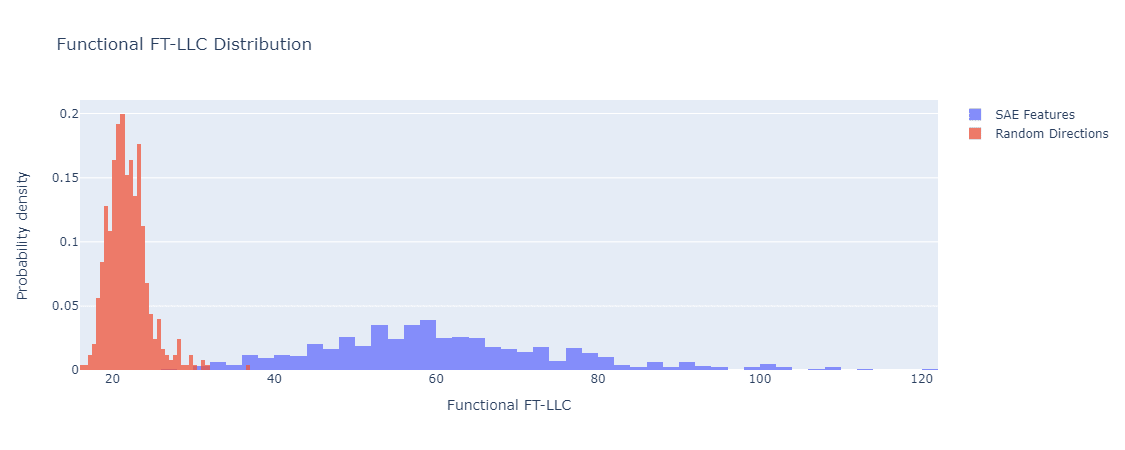
Functional FT-LLC of random directions vs. SAE features. GPT-2-small residual stream layer 9.

We can see that the distributions seem to have a nice Gaussian shape, with some outlier samples. Moreover, They seem to be well separated. The estimates we get for the means, standard deviations, and $\delta$ are:

$$\begin{array}{cc}& {\mu }_{\text{rand}}=21.90,{\sigma }_{\text{rand}}=2.51\\ & {\mu }_{\text{sae}}=60.67,{\sigma }_{\text{sae}}=15.24\\ & \delta =0.4\%\end{array}$$

Also, note that $0.4\%$ is a very small number when taking into account that we use only $500$ samples for each of the random direction and SAE features. In fact, this means only $4$ samples are misclassified by the corresponding threshold-based classifier, which is too small a number to give a good estimate. We plan to perform larger experiments and produce more exact estimations.

It is worth noting that we haven't tried to optimize these numbers yet, for example by spending more compute on the estimation or analyzing pathological cases leading to outliers.

Behavioral FT-LLC The figure below shows the distributions of Behavioral FT-LLC estimates for $500$ random directions in layer $9$ of GPT-2-small vs. $500$ SAE features in the same. The feature corresponding to each direction is the linear projection onto it.

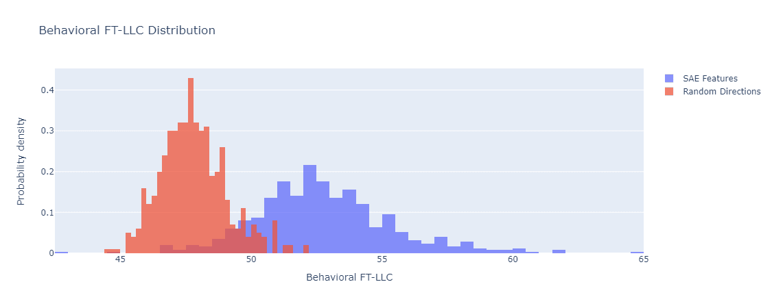
Behavioral FT-LLC of 500 random directions vs. $500$ SAE features. GPT-2-small residual stream layer 9.

Here the distributions have a Gaussian shape as well, but the separation is significantly less pronounced (although clearly exists). The estimates for the means, standard deviations, and $\delta$ are:

$$\begin{array}{cc}& {\mu }_{\text{rand}}=47.80,{\sigma }_{\text{rand}}=1.26\\ & {\mu }_{\text{sae}}=52.74,{\sigma }_{\text{sae}}=2.66\\ & \delta =8.5\%\end{array}$$

Comparison to other metrics

We compare our results with similar experiments done on ablation-based metrics. Out of all the metrics we tried, only one separated features and random directions comparably well to the functional FT-LLC. We also provide below sparsity distributions for our features and random directions, mainly as a sanity check that the performance of FT-LLC is not due to sparsity effects.

Sparsity Metrics

Sparsity The figure below shows the distribution of the sparsity, i.e. the probability of the thresholded feature to be zero. thresholds are set to one standard deviation of each feature's activations.

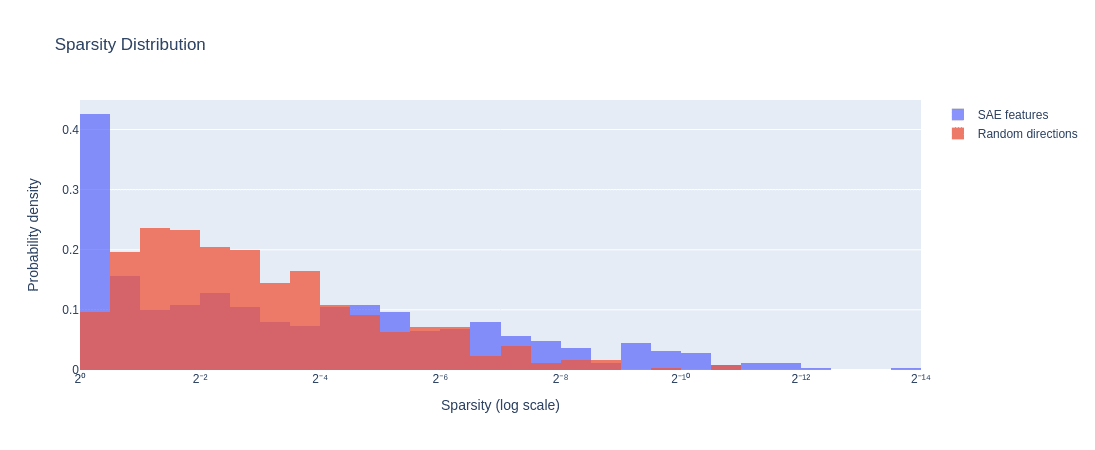
Sparsity of 500 random directions vs. 500 SAE features. GPT-2-small layer 9.

Norm Sparsity Since functional FT-LLC computes features on all the tokens of the input as one unit (opposed to, for example, averaging over the result for each token) we also checked the sparsity of activation norm where activation here is with respect to all token positions together. Thus, for each feature the norm reduces a tensor of shape $(\text{batch dim},\text{token dim})$ (our features are one dimensional) to a tensor of shape $\left(\text{batch dim}\right)$. The figure below shows the distribution of the sparsity of the activation norm.

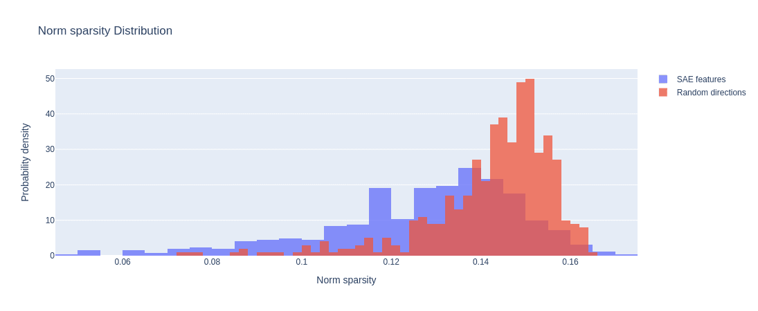
Norm sparsity of 500 random directions vs. 500 SAE features. GPT-2-small layer 9.

Ablation Influence

We experimented with using ablation-effect based metrics to distinguish features from random directions. For each direction, we tried ablating the value of the feature to $0$ or to its mean value across our dataset, measuring both the KL divergence from the undisturbed model and the sparsity of the divergence (as was done here), either taking the average over the entire dataset or only over the $k$ data-points with the strongest activations, for various values of $k$.

We found, as expected, that taking the top $k$ activations yield significantly better separation than averaging over all data points. Also, mean-ablation yields significantly better results than zero-ablation for KL divergence, but slightly worse results for sparsity.

The figures below show the distributions of the ablation effect KL divergence and sparsity, each with the parameters that provided the best separation. The separation metrics are $\delta =1\%$ for KL divergence and $\delta =4.6\%$ for sparsity.

Here, similarly to the situation with the functional FT-LLC, note that $1\%$ means only $10$samples are misclassified.

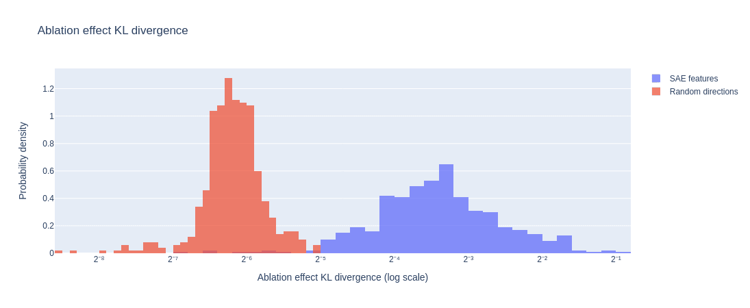
Mean-ablation effect KL divergence of 500 random directions vs. 500 SAE features, evaluated on the top-16 activations for each direction. GPT-2-small layer 9.

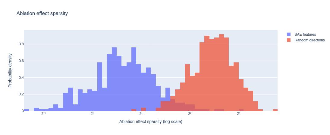
Zero-ablation effect sparsity of 500 random directions vs. 500 SAE features, evaluated on the top-$8$ activations for each direction. The sparsity measure is L1/L2. GPT-2-small layer 9.

Best vs. Best: Top-16 Mean-Ablation and $1\sigma$ Functional FT-LLC

Finally, we checked the relationship between the best ablation-based method and best LLC based-method. Namely, Top-16 Mean-Ablation and $1\sigma$ Functional FT-LLC. The figure below shows the two metrics against each other.
The correlation matrix for the two metrics for SAE features and random directions are:

$${\rho }_{\text{rand}}=0.38$$$${\rho }_{\text{sae}}=0.47$$

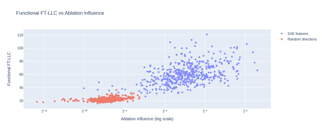
Top-16 mean-ablation and 1$\sigma$ functional FT-LLC. 500 random directions vs. 500 SAE features. GPT-2-small layer 9.

It seems from looking at the graph that the correlation for random directions
is mostly due to samples with metrics tending to values typical of SAE features, which might suggest that these directions are close enough to a feature (not necessarily amongst our SAE features) and the metrics reflect that. Indeed, when restricting ourselves to samples which are below-median by the measures, the correlation effectively vanishes.

However, one could wonder why the metrics would be correlated, for features, in the first place? One of the metrics measures a notion of complexity of computing a feature which is dependent on the weights before the layer of the feature, while the other measures the influence of ablating the feature on the output, which is dependent on the computation done after the corresponding layer.

We have two theories regarding this correlation. The first suggests that the correlation is a reflection of imperfect features. That is, the features we find using the SAE are imperfect approximations of true features — either true directions in the model or some ideal true features that are only approximately represented as thresholded linear projections. Thus, SAE features that are better approximations tend to get higher functional FT-LLC values and higher ablation influence values.

Another theory suggests that features with higher ablation influence are more important for the overall computation and so it is efficient for the model to invest more weight space volume in their computation. Note that the two theories are not contradictory. We are working on clarifying this point and expect to have more to say in our next posts.

Overall takes

All in all, our results significantly updated us towards believing this agenda warrants a deeper study. Both statistical properties of feature activations and ablation interventions seem unable to fully explain or recover the feature identification properties offered by FT-LLC (at least the alternatives we tried). We are now more optimistic both with regard to the ability to arrive at meaningful estimates with reasonable resources and the validity of our overall approach. However, we are not yet convinced that our motivations can be achieved and in order to address this concern we are working on:

1. Verifying the results generalize to other settings.
2. Developing a theoretical basis to explain them.
3. Analyzing particular cases (SAE features with random like FT-LLC estimates, out of distribution FT-LLC estimates etc.) to see if we can understand them.

We work on these while also further investigating the use of LLC estimations on model internals. See the next section for more details.

Further Directions

Given the findings we have got there is much work yet to be done:

Verification and amplification of our findings: do our findings generalize to other models? Other FT-LLC variants? Other SAEs? Can the results for the behavioral FT-LLC be sharpened? Can we understand FT-LLC outliers?

A more detailed investigation: one can delve deeper in analyzing our results. On top of the directions we mentioned in the post one could, for example, study cross-layer relationships of FT-LLC estimates. Another direction would be to study the influence of different data points on the estimate and its relationship with the activation values of the feature on those data points.

Feature quality metric: can some FT-LLC variant be used as a reliable quality metric? Are SAE-predicted features with random like estimates actual features of the model? On the other side, are features with non-random estimates actual features of the model? Can we find random directions with feature like FT-LLC estimates?

Theory: develop the mathematical theory behind our findings. Of particular interest to us is whether we can describe (and derive constraints on) the structure of the set of directions with phenomenal FT-LLC.

We have already started investigating the directions above. Further directions include the use of FT-LLC estimation for feature identification and as a developmental metric, but we think a more comprehensive understanding of more basic questions is needed before pursuing these directions.

Prior Work

We are unaware of previous work applying LLC estimation to model internals' alterations. Below we list works which introduce or share several of the components of our strategy or have similar motivations.

Sparse Autoencoders

By now there is already a significant body of work on sparse autoencoders and their variants. Works on the forum can be found here [? · GW]. Note that from the point of view of studying FT-LLC as a general feature quality metric sparse autoencoders mainly serve as an approximate ground truth for features to study and iterate on.

Singular Learning Theory and Developmental Interpretability

The idea to use singular learning theory, and in particular LLC estimation, for interpretability purposes is far from new. As far as we are aware the most common agenda which is related to our project is Developmental Interpretability, which aims to identify phase transitions (developmental stages) during the training of the model and use these to identify meaningful structures learned during the phase transition. These phase transitions are identified by analyzing the trajectory of the weights in weight space and the change of LLC estimates and loss during training (for example, this work). In particular, LLC estimation is done on the entire model, using loss functions on the output. In contrast, our approach uses only the final weights of the model and utilizes LLC estimations of alterations of the model with different loss functions.

Another work related to ours is this one, which is heavily inspired by SLT. Here the authors aim to find features using the final weights of the model (note that in this exploratory post we haven't addressed feature finding yet). However, their method is very different from ours: it uses gradients and activations directly and appeals to global structures, not individual directions.

Acknowledgements

We'd like to thank Daniel Murfet for a helpful discussion and feedback on our work. 
I (Lidor) would like to thank Lee Sharkey for his guidance during my first steps in interpretability research, and for pointing me towards singular learning theory as an interesting approach to interpretability.

Authors Contribution Statement

Lidor came up with and initiated the project, wrote the codebase and ran LLC estimations and calibration sweeps. Aviel added features to, debugged and ran the ablation experiments. We analyzed and discussed the results together. Lidor wrote most of this post, with Aviel writing some parts.

1. ^{^}

   Usually one dimensional (thresholded) projections, but sometimes higher dimensional functions.

2. ^{^}

   Though it is used in related settings, such as circuit identification, and thus can be used indirectly as a quality metric through these uses.

3. ^{^}

   The following generalizes to functions with higher output dimension verbatim, but this is the setting we focus on in this post.

4. ^{^}

   This is related to saddle points, for example see this for a discussion in the context of deep linear networks.

5. ^{^}

   More popularly known as phase transitions, though the emphasis is different - in particular with respect to the suddenness of the transition.

6. ^{^}

   Some SAEs variants do get exposed to more data than what is encapsulated in layer activations, but not the one we use.

6 comments

Comments sorted by top scores.