SAE Dataset Sensitivity in Feature Matching and a Hypothesis on Position Features

post by Seonglae Cho (seonglae) · 2025-02-26T17:05:18.265Z · LW · GW · 0 comments

Contents

  Abstract
  1. Introduction
  2. Preliminaries
      2.1 Mechanistic Interpretability
      2.2 Residual Stream
      2.3 Linear Representation Hypothesis
      2.4 Superposition Hypothesis
      2.5. Sparse Autoencoder
  3. Method
    3.1. Feature Activation Visualization
    3.2. Feature and Neuron Matching
  4. Results
    4.1. Analysis on Feature Activation
      4.1.1. Feature Activation across Token Positions
      4.1.2. Feature Activation with Quantiles
    4.2. Analysis on Feature Matching
      4.2.1 Feature and Neuron Matching
      4.2.2 Effect of Training Settings on Feature Matching
      4.2.3 Feature Matching along the layers
  5. Conclusion
  6. Limitation
  7. Future works
  8. Acknowledgments
  9. Appendix
      9.1. Implementation Details
      9.2. Activation Average versus Standard Deviation
      9.4. LLM Loss and SAE Loss
      9.5 UMAPs of feature directions
      9.6. Trained SAEs options
    Additional Comments
None
No comments

Abstract

Sparse Autoencoders (SAEs) linearly extract interpretable features from a large language model's intermediate representations. However, the basic dynamics of SAEs, such as the activation values of SAE features and the encoder and decoder weights, have not been as extensively visualized as their implications. To shed light on the properties of feature activation values and the emergence of SAE features, I conducted two distinct analyses: (1) an analysis of SAE feature activations across token positions in comparison with other layers, and (2) a feature matching analysis across different SAEs based on decoder weights under diverse training settings. The first analysis revealed potentially interrelated phenomena regarding the emergence of position features in early layers. The second analysis initially observed differences between encoder and decoder weights in feature matching, and examined the relative importance of the dataset compared to the seed, SAE type, sparsity, and dictionary size.

1. Introduction

The Sparse Autoencoder (SAE) architecture, introduced by Faruqui et al., has demonstrated the capacity to decompose interpretable features in a linear fashion (Sharkey et al., 2022 [LW · GW]; Cunningham et al., 2023; Bricken et al., 2023). SAE latent dimensions can be interpreted as monosemantic features by disentangling superpositioned neuron activations from the LLM's linear activations. This approach enables decomposition of latent representations into interpretable features by reconstructing transformer residual streams (Gao et al., 2024), MLP activations (Bricken et al., 2023), and even dense word embeddings (O'Neill et al., 2024).

SAE features not only enhance interpretability but also function as steering vectors (White, 2016; Subramani et al., 2022; Konen et al., 2024) for decoding-based clamp or addition operations (Durmus et al., 2024; Chalnev & Siu, 2024). In this process, applying an appropriate coefficient to the generated steering vector is crucial for maintaining the language model within its optimal "sweet spot" without breaking it (Durmus et al., 2024). Usually, quantile-based adjustments (Choi et al., 2024) or handcrafted coefficients have been used to regulate a feature’s coefficient. For future dynamic coefficient strategies, to improve efficiency in this regard, it is necessary to examine how feature activation values are distributed under various conditions.

Despite the demonstrated utility of SAE features, several criticisms remain, one being the variability of the feature set across different training settings. For instance, Paulo & Belrose show that the feature set extracted from the same layer can vary significantly depending on the SAE weight initialization seed. Moreover, SAEs are highly dependent on the training dataset (Kissane et al., 2024 [LW · GW]), and there is even some doubt that a randomly initialized transformer tends to extract primarily single-token features that might describe the dataset more than the language model itself (Bricken et al., 2023; Paulo & Belrose, 2025). Ideally, it is crucial to robustly distinguish LLM-intrinsic features from dataset artifacts, making it critical to assess the impact of various factors on SAE training.

In this work, I first visualize how feature activations manifest in a trained SAE across different layers and token positions to understand their dynamics. Then, by training SAEs under various training settings and applying feature matching techniques (Balagansky et al., 2024; Laptev et al., 2025; Paulo & Belrose, 2025), I compare the similarity of the extracted feature sets through the analysis of decoder weights. This work aims to (1) efficiently discover onboard SAE features by visualizing the distribution of feature and activation values without requiring extensive manual intervention, and (2) compare the relative impact of different training settings on the feature transferability across the same residual layers under diverse conditions.

2. Preliminaries

2.1 Mechanistic Interpretability

Mechanistic Interpretability seeks to reverse-engineer neural networks by analyzing their internal mechanisms and intermediate representations (Neel, 2021; Olah, 2022). This approach typically focuses on analyzing latent dimensions, leading to discoveries such as layer pattern features in CNN-based vision models (Olah et al., 2017; Cartern et al., 2019) and neuron-level features (Schubert et al., 2021; Goh et al., 2021). The success of the attention mechanism (Bahdanau et al., 2014; Parikh et al., 2016) and the Transformer model (Vaswani et al., 2017) has further spurred efforts to understand the emergent abilities of transformers (Wei, 2022).

2.2 Residual Stream

In transformer architectures, the residual stream, as described in Elhage et al., is a continuous flow of fixed-dimensional vectors propagated through residual connections. It serves as a communication channel between layers and attention heads (Elhage et al., 2021), making it a focal point of research on transformer capabilities (Olsson et al., 2022; Riggs, 2023 [LW · GW]).

2.3 Linear Representation Hypothesis

In the vector representation space of neural networks, it is posited that neural networks exhibit linear directions in activation space (Mikolov et al., 2013). This has led to studies demonstrating that word embeddings reside in interpretable linear subspaces (Park et al., 2023) and that LLM representations are organized linearly (Elhage et al., 2022; Gurnee & Max Tegmark, 2024). This hypothesis justifies the use of inner products, such as cosine similarity, directly in the latent space; in addition, Park et al., 2024 have proposed alternatives like the causal inner product.

2.4 Superposition Hypothesis

In neural network representations, the superposition of thought vectors (Goh, 2016) and word embeddings (Arora et al., 2018) provided empirical evidence of superposition in neural networks' representations. Using toy models, Elhage et al. detailed the emergence of the superposition hypothesis through the process of phase change in feature dimensionality, linking it to compressed sensing (Donoho, 2006; Bora et al., 2017). Additionally, transformer activations are empirically found to exhibit significant superposition (Gurnee et al., 2023). While this superposition effectively explains the operation of LLMs, its linearity remains a controversial topic (Mendel, 2024 [LW · GW]).

2.5. Sparse Autoencoder

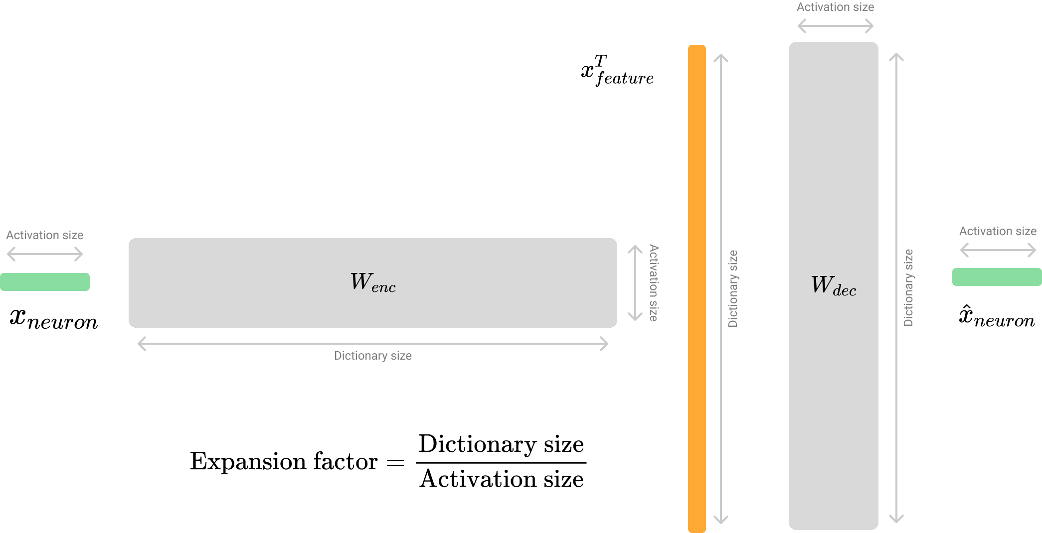
Residual SAE takes the residual vector from the residual stream as input. Here, the term neuron refers to a single dimension within the residual space, while feature denotes one interpretable latent dimension from the SAE dictionary. The SAE reconstructs the neurons through the following process. ^[1]

$$x_{feature}=Activation(x_{neuron}\cdot W_{enc}+b_{enc})$$$${\hat{x}}_{neuron}=x_{feature}\cdot W_{dec}+b_{dec}$$

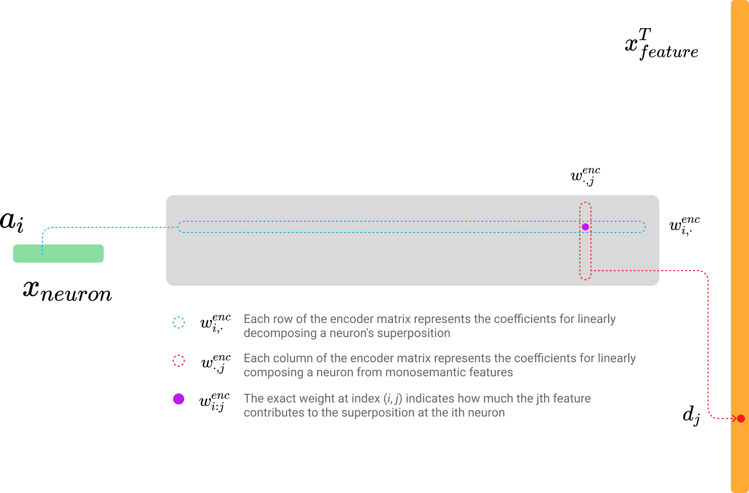
The encoder weight matrix multiplication can be represented in two forms that yield the same result:

$$x_{feature}=Activation\left(\sum _i^A\right(a_i\cdot w_{i,\cdot }^{enc})+b_{enc})$$$$x_{feature}=Activation\left(\underset{i}{\overset{D}{⨁}}\right(x_{neuron}\cdot w_{\cdot ,j}^{enc}+b_j^{enc}\left)\right)$$

where $A$ is the activation size and $D$ is the dictionary size and $⨁$ denotes group concatenation.

• $w_{i,\cdot }^{enc}$: Each row of the encoder matrix represents the coefficients for linearly disentangling a neuron's superposition.
• $w_{\cdot ,j}^{enc}$: Each column of the encoder matrix represents the coefficients for linearly composing a neuron from monosemantic features.
• $w_{i:j}^{enc}$: The specific weight at index $(i,j)$ indicates how much the $j$th feature contributes to the superposition at the $i$th neuron.

As shown in the images above and below, each row and column of the encoder and decoder plays a critical role in feature disentanglement and neuron reconstruction.

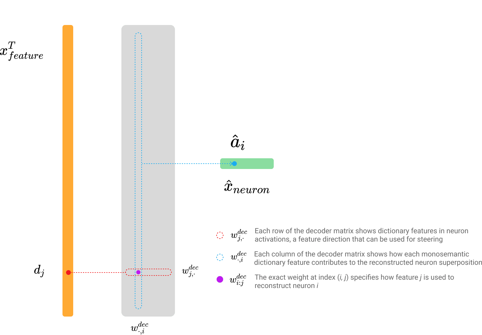
The decoder weight matrix multiplication can also be represented in two forms that yield the same result:

$${\hat{x}}_{neuron}=\sum _j^D(d_j\cdot w_{j,\cdot }^{dec}+b_j^{dec})$$$${\hat{x}}_{neuron}=\underset{i}{\overset{D}{⨁}}(x_{feature}\cdot w_{\cdot ,i}^{dec})+b_{dec}$$

• $w_{j,\cdot }^{dec}$: Each row of the decoder matrix shows dictionary features in neuron activations, a feature direction (Templeton, 2024) that can be used for steering.
• $w_{\cdot ,i}^{dec}$: Each column of the decoder matrix shows how each monosemantic dictionary feature contributes to the reconstructed neuron superposition.
• $w_{j:i}^{dec}$: The specific weight at index $(i,j)$specifies how feature $j$ is composited (Olah, 2023) to reconstruct neuron $i$.

This formulation underscores the critical role of both encoder and decoder weights in disentangling features and accurately reconstructing neuron activations. Correspondingly, early-stage SAEs were often trained with tied encoder and decoder matrices (Cunningham et al., 2023 [AF · GW]; Nanda, 2023 [AF · GW]). By the same reasoning, the decoder weights are commonly used for feature matching (Balagansky et al., 2024; Laptev et al., 2025; Paulo & Belrose, 2025) because they capture the feature direction (Templeton, 2024).

3. Method

3.1. Feature Activation Visualization

The feature activation (indicated by the red point in Figures 3 and 4) is a core component of the SAE, serving as the bridge between neurons and features via the encoder and decoder. I visualized the feature activation distributions, including quantile analyses, to capture patterns like related studies(Anders & Bloom, 2024 [LW · GW]; Chanin et al., 2024).

First, I examined overall feature distribution and the changes in activation values across token positions. Due to the well-known attention sine phenomenon (Xiao et al., 2023), even after excluding the outlier effects of the first token, both the quantile-based averages and token-position averages were computed. Finally, to capture the dynamics of feature set along the layer dimension, I visualized the quantile distribution.

Specifically, the analysis comprises the following five components:

1. Feature Activation Average across Token Positions
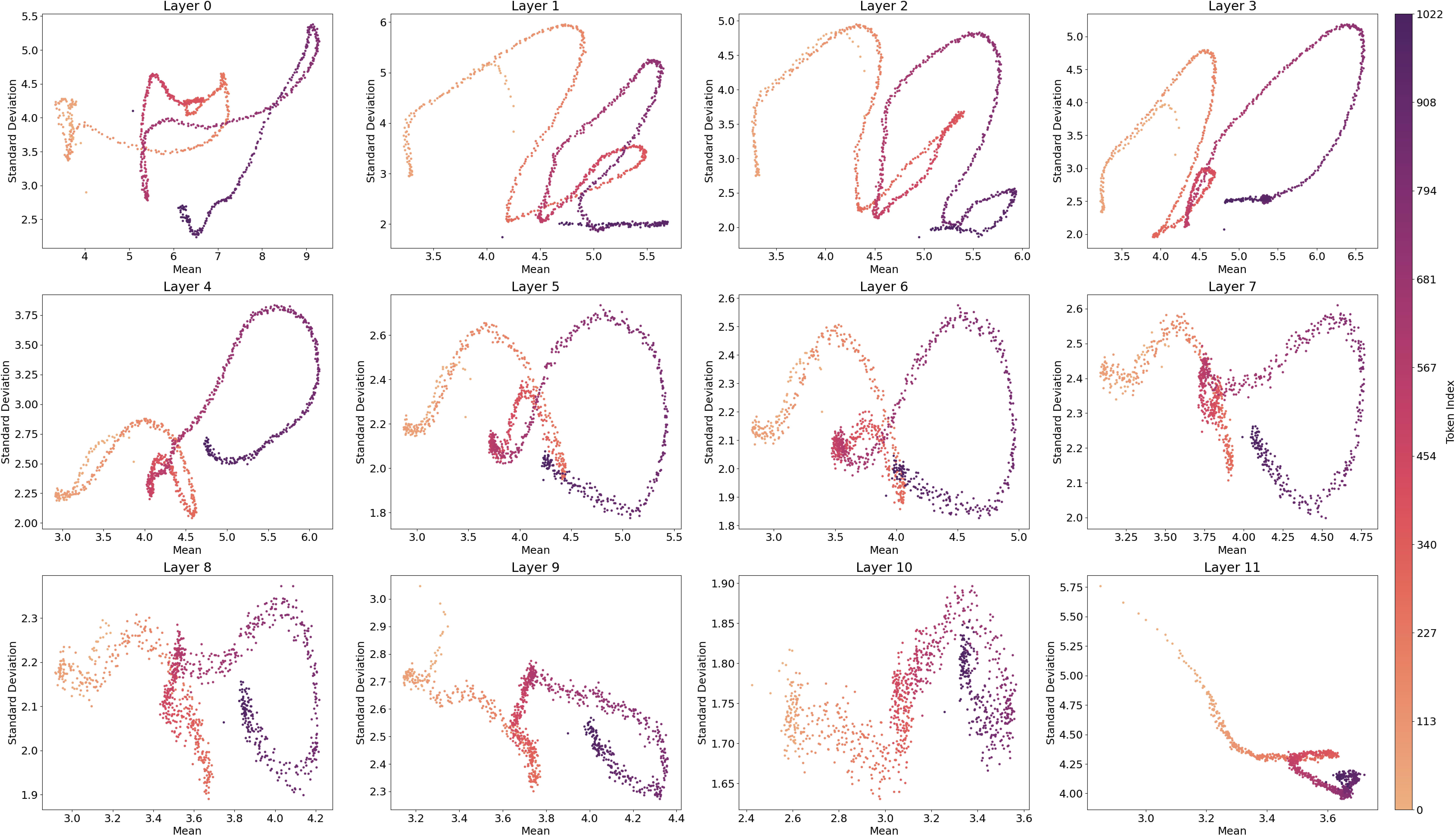
2. Token Average and Token Standard Deviation
3. Feature Average and Feature Standard Deviation
4. Feature Average and Feature Density
5. Decile Levels for Each Feature

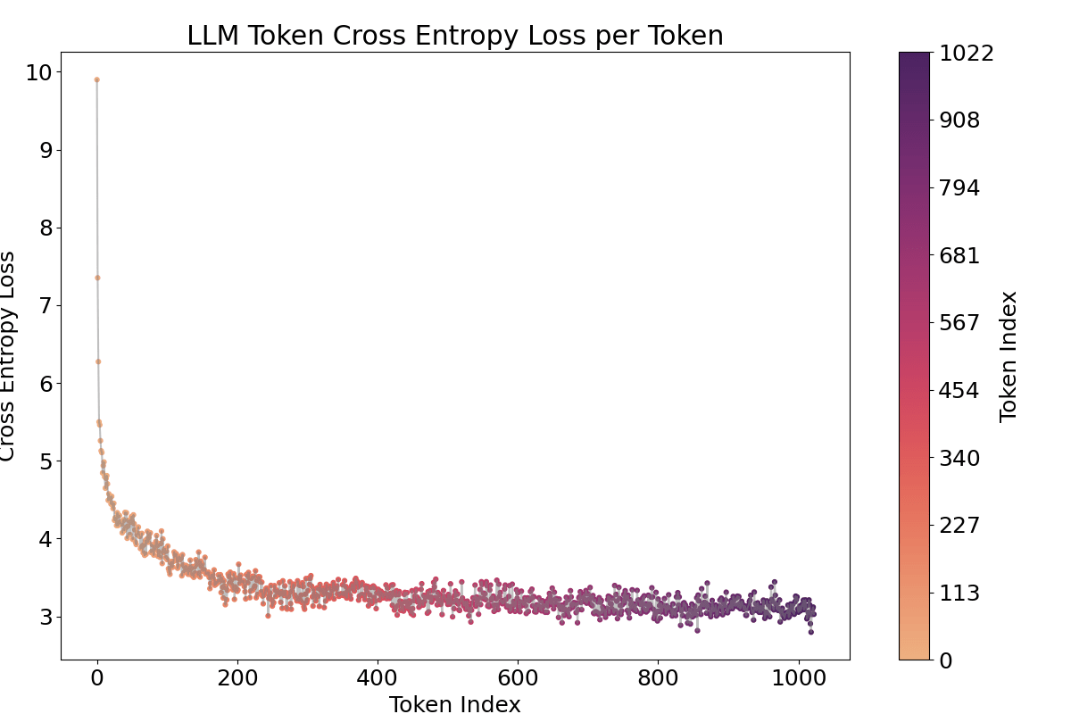
To validate these results, several evaluation metrics were presented. The trends of the LLM's cross-entropy, as well as the SAE's reconstruction MSE (L2 loss) and L1 loss, are detailed in the appendix.

3.2. Feature and Neuron Matching

Previous studies have suggested that SAEs may simply capture dataset-specific patterns (Heap et al., 2025) or that SAE training is highly sensitive to initialization seed (Paulo & Belrose, 2025). To assess the sensitivity of the feature set to variations in seed, dataset, and other SAE training settings, I formulated the following hypothesis.

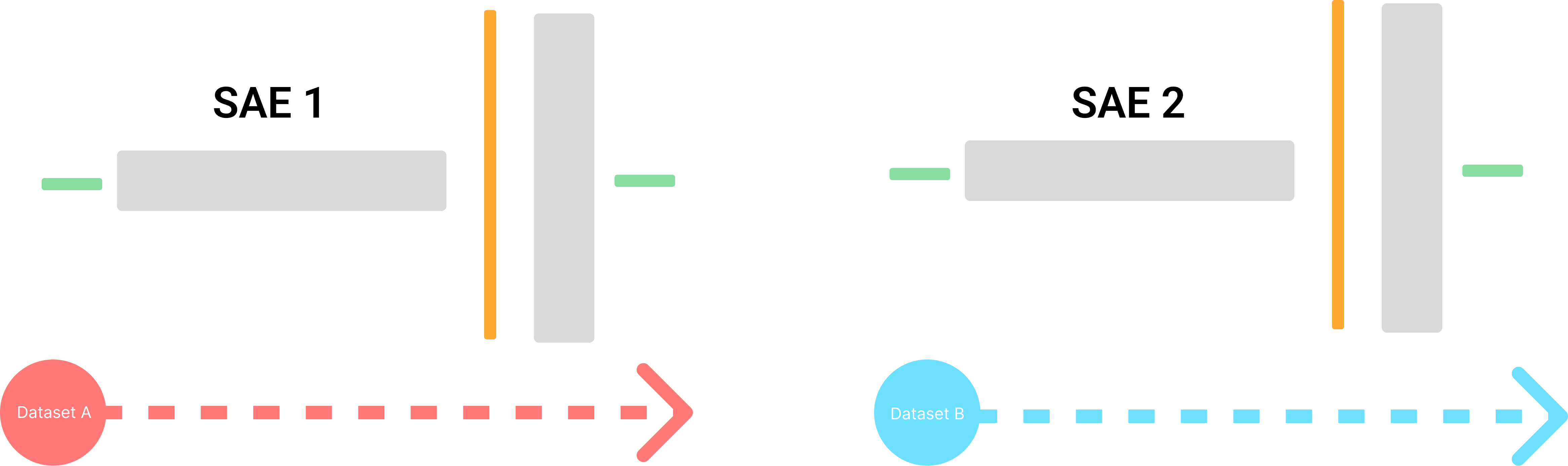
In an ideal scenario, SAEs trained under different settings should recover the same feature set, they should learn the same feature set, even if separate SAEs are trained under different settings such as the training dataset and initialization seed.

Let $d_j\in D_1$ denote a feature in the dictionary $D_1$ from SAE1, and $d_k^{\prime }\in D_2$ denotes a feature in the dictionary $D_2$ from SAE2. If $d_j$ and $d_k^{\prime }$ represent the same monosemantic feature extracted from the LLM, they should exhibit similar compositional and superpositional properties in their respective weight matrices.

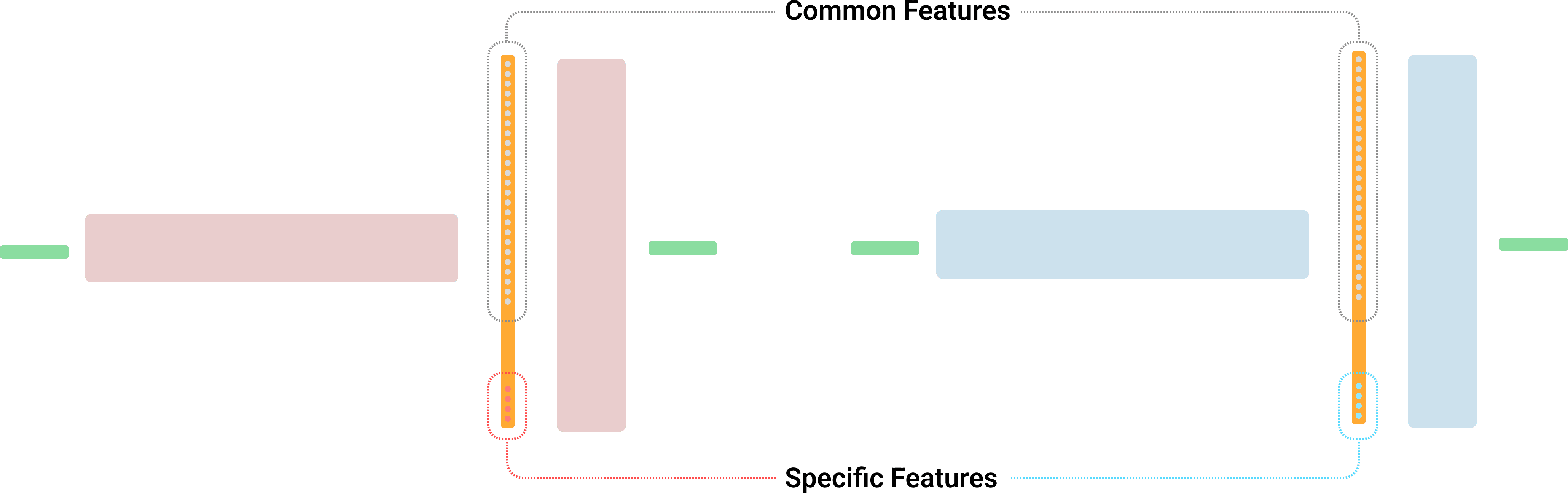
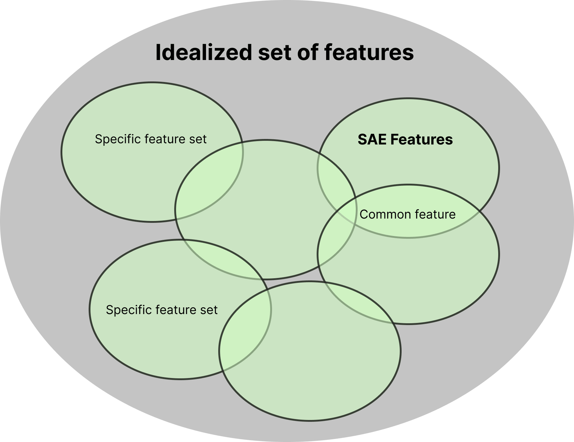
However, as Zhong & Andreas noted, SAEs often capture dataset-specific patterns in addition to features intrinsic to LLMs. Consequently, as illustrated in Figure 6, each SAE is expected to learn certain specific (or "orphan") features unique to its training setting (Paulo & Belrose).

Between two primary approaches to feature matching, as outlined by Laptev et al. (2025), I chose the second decoder weight-based analysis.

• Causal Effect Measurement: Assess correlations between activations to measure causal effects (Wang et al., 2024; Balcells et al., 2024)
• Direct Weight Comparison: Directly compare SAE feature weights $w_{\cdot ,j}^{enc}$ or $w_{j,\cdot }^{dec}$ for cost-efficiency (Dunefsky et al., 2024; Balagansky et al., 2024).

The second geometric approach is suitable for across diverse settings for this experiment and demonstrated the ability to measure features on mean maximum cosine similarity (MMCS) proposed by Sharkey et al. (2022) [AF · GW]. Under the linear representation hypothesis, calculating the inner product (i.e., cosine similarity) allows us to gauge the degree of feature matching (Park et al., 2023). Thus, I compute cosine similarity values for each SAE feature weight and apply a threshold ${\tau }_{feature}$ to the highest similarity value. If the highest similarity exceeds ${\tau }_{feature}$, the feature is considered common; otherwise, it is deemed specific.

$$m_j=\underset{w_k^{\prime }\in W_2}{max}\frac{w_j\cdot w_k^{\prime }}{\parallel w_j\parallel \parallel w_k^{\prime }\parallel }$$$$\text{Feature Type}\left(d_j\right)=\{\begin{array}{cc}\text{common}& \text{if}{m}_j\ge {\tau }_f,\\ \text{specific}& \text{if}{m}_j<{\tau }_f.\end{array}$$

I computed the cosine similarity for each SAE feature's weight (using the rows of the Decoder, where $w_j=w_{j,\cdot }^{dec}$) to compare features. In addition to this standard analysis, I also explored matching via Encoder column analysis (when $w_j=w_{\cdot ,j}^{enc}$), as discussed in Figures 3 and 4, and via matching between Encoder rows and Decoder columns. In that case, let $a_i\in N_1$ denote a neuron in the neuron set $N_1$ from SAE1, and $a_l^{\prime }\in N_2$ denote a neuron in the neuron set $N_2$ from SAE2. These neurons were analyzed in a similar manner to features , using a threshold ${\tau }_{neuron}$ and weight vectors $w_i\in \{w_{i,\cdot }^{enc},w_{\cdot ,i}^{dec}\}$.

$$m_i=\underset{w_l^{\prime }\in W_2}{max}\frac{w_i\cdot w_l^{\prime }}{\parallel w_i\parallel \parallel w_l^{\prime }\parallel }$$$$\text{Neuron Type}\left(a_i\right)=\{\begin{array}{cc}\text{common}& \text{if}{m}_i\ge {\tau }_n,\\ \text{specific}& \text{if}{m}_i<{\tau }_n.\end{array}$$

While the Hungarian algorithm (Kuhn, 1955) is commonly used for one-to-one feature matching to compute exact ratios, here I focus on the relative impact of training options. In this framework, a higher feature matching score among SAEs of the same layer indicates a greater overlap of shared common features and higher feature transferability across different training settings. Conversely, a lower matching score suggests a larger proportion of specific features, implying lower transferability under changed training conditions.

4. Results

4.1. Analysis on Feature Activation

In this experiment, I began by aligning observations from previous studies on the final layer and then extended the analysis across multiple layers. This approach was applied to two different GPT2-small SAEs over all 12 layers: one using an open-source ReLU-based minimal SAE (Bloom, 2024 [LW · GW]) and the other a Top-k activated SAE (Gao et al., 2024), enabling a direct comparison between the two.

For visualization clarity, I employed a consistent color palette for each dimension:

• Token Position: mapped to the flame palette
• Layer Index: mapped to the viridis palette (as in Anders & Bloom, 2024 [LW · GW])
• Quantile Level: mapped to the   mako palette

4.1.1. Feature Activation across Token Positions

It is well known that the activations of the first and last tokens tend to be anomalous due to the “attention sink” effect (Xiao et al., 2023). As expected, Figure 7 shows that the first token exhibits a higher activation value.^[2]

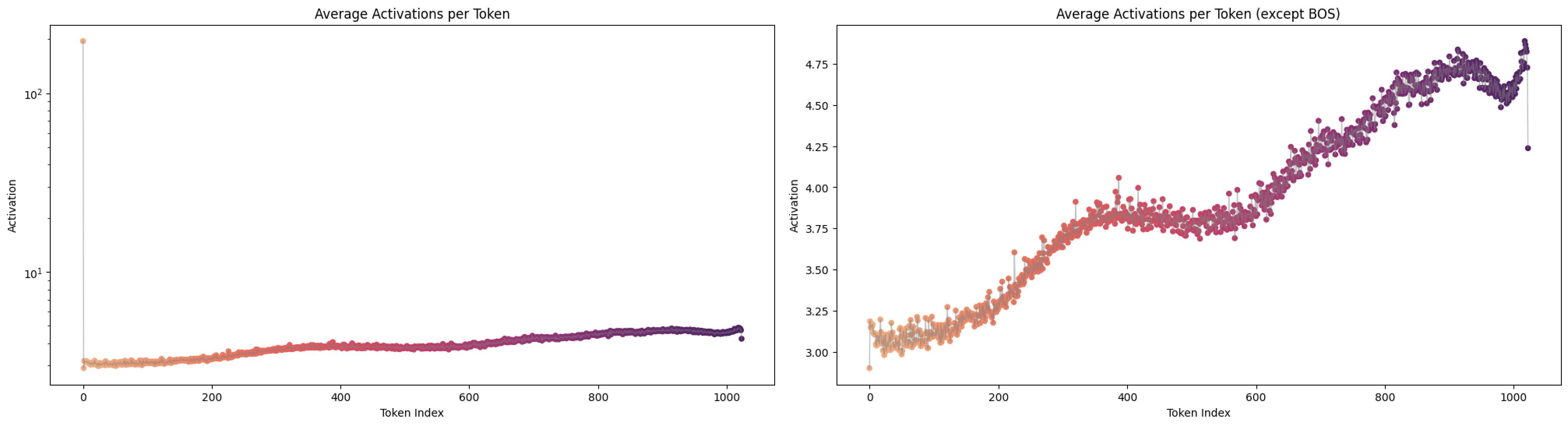
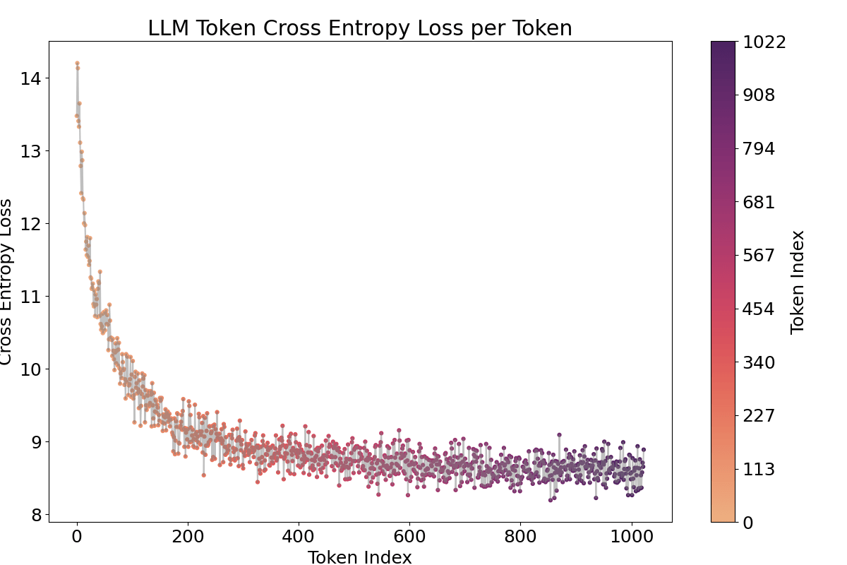
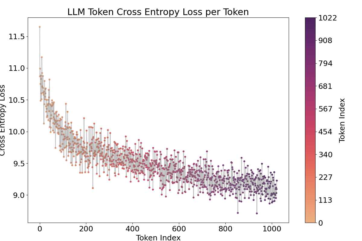
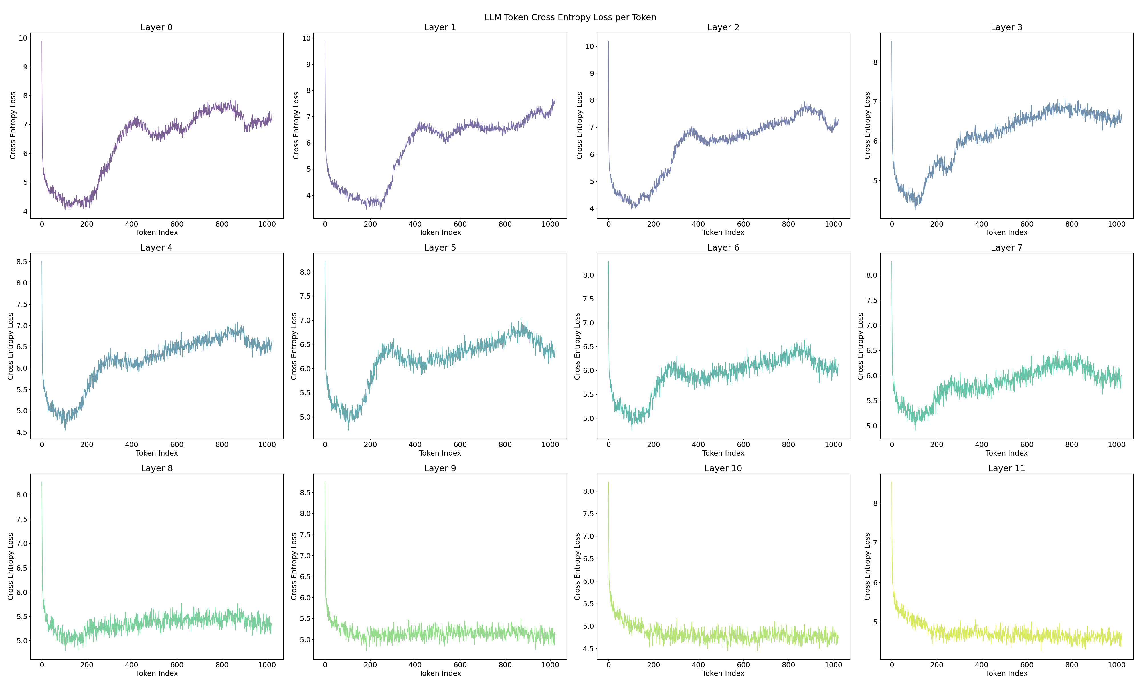
A notable observation is the fluctuating pattern of activation averages along the token positions. This finding supports Yedidia (2023) [LW · GW] discovery that GPT2-small’s positional embedding forms a helical structure, roughly two rotations are visible in the visualization. For a more detailed analysis across all layers, and to mitigate the attention sink effect through input/output normalization(Gao et al., 2024), I trained a Top‑k SAE (instead of a ReLU-based one) on all 12 layers of GPT2‑small where the loss graphs are at Figure 16.^[3]

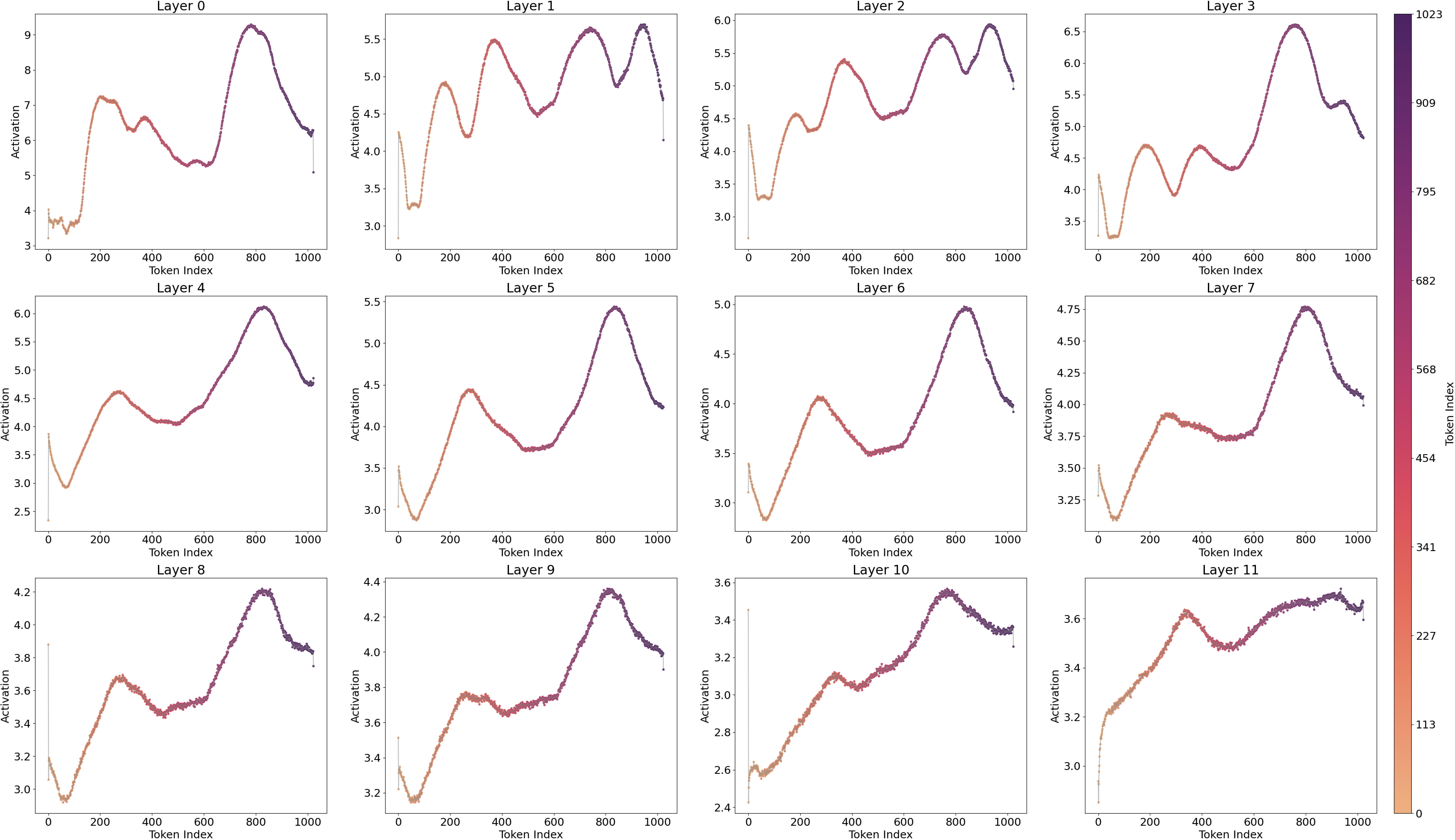
To address these issues, I trained the Top-k SAE with input normalization (Gao et al., 2024), a method that proved more robust than the ReLU SAE, yielding significantly lower loss and cross-entropy differences. In above Figure 8, the overall visualization (except for layers 1–3) displays a two-period oscillation like a signomial function could be linearly projected from helical structure. However, layers 1–3 show four fluctuations, suggesting a multiple of the original base frequency, which raises the question of whether an operation is effectively doubling the frequency. This possibility will be explored in the next section.

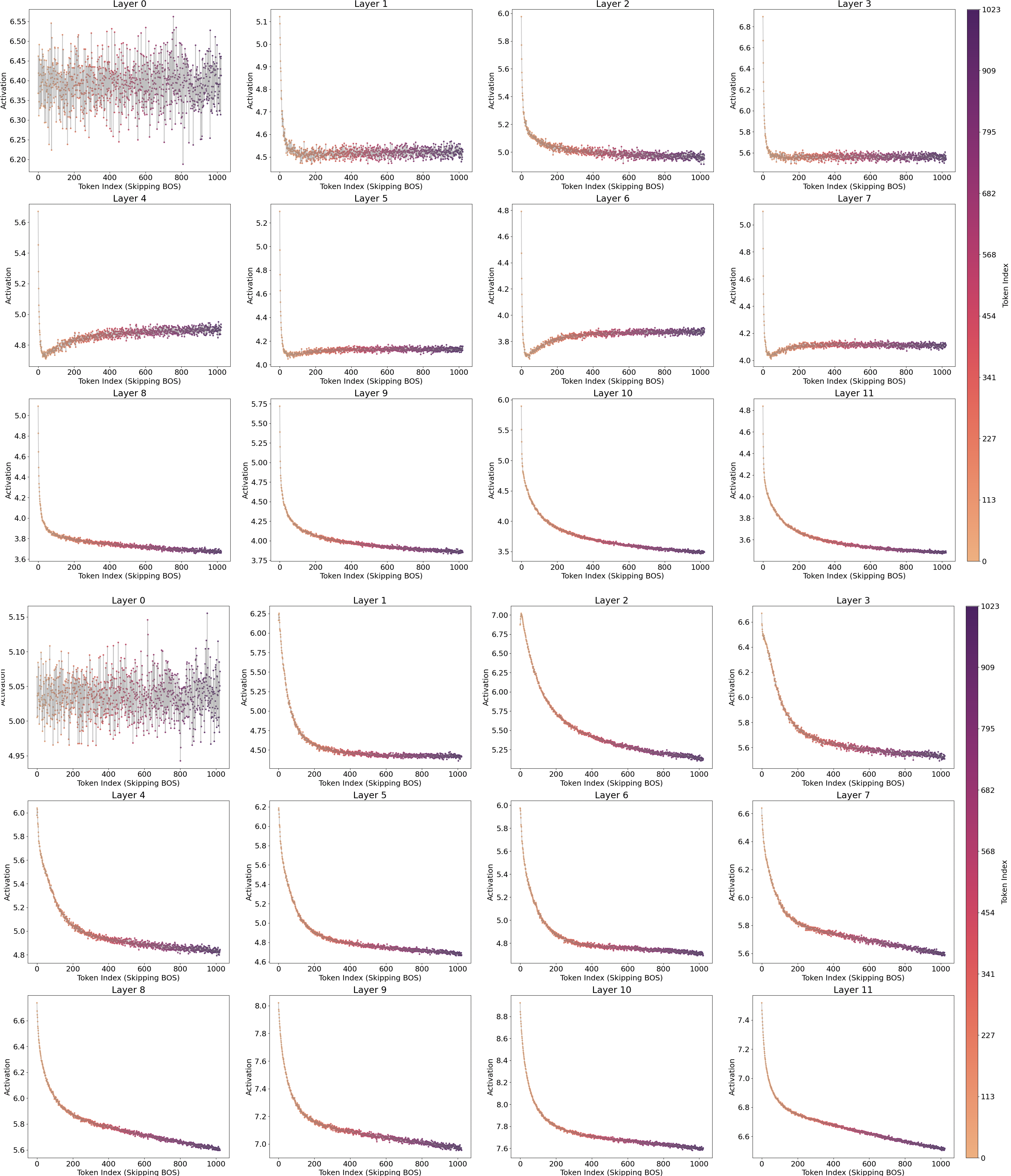
One piece of evidence supporting that this activation fluctuation is caused by the positional embedding is that when we ablate or shuffle the positional encoding, the pattern vanishes. I either ablated the positional encoding (setting it to zero) or shuffled it for 1024 positions, the repeated pattern across tokens vanished, even though obviously confusing positions in both methods led to increased cross-entropy and SAE loss as shown in the Appendix Figure 15, 17. Shuffled method showed less loss increase. Furthermore, the language model’s capability to process sequences up to 1024 tokens is demonstrated by the decreasing cross-entropy in Figure 19. 

4.1.2. Feature Activation with Quantiles

In this section, I examine the features in terms of quantiles to better understand their roles in feature steering and feature type classification, linking these observations with previous findings.

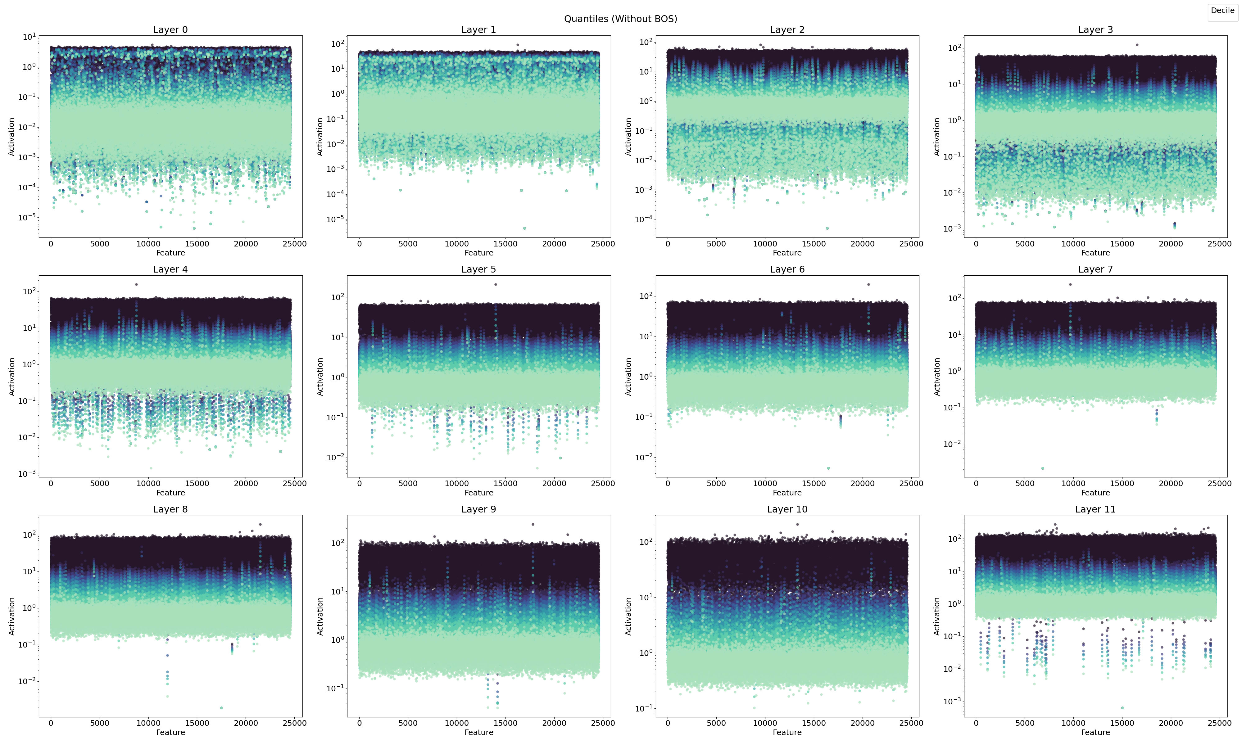
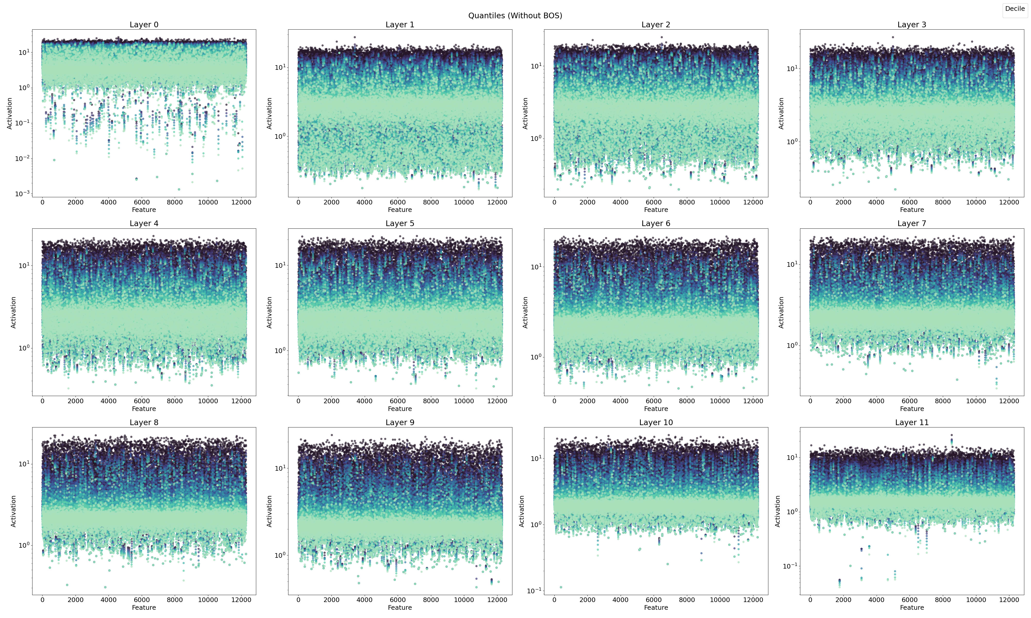
In Figure 10, the ReLU SAE reveals two distinct feature sets, one with high activations and one with low activations, particularly in the early layers (0–3). Combining this observation with previous results, I hypothesize a connection between the positional neurons described by Gurnee et al., (2024) and the position features identified in layer 0 by Chughtai & Lau, (2024) [LW · GW], which appear to emerge in the early stages of the network.

To summarize, three key aspects emerge:

• Position Features: As reported by Gurnee et al. (2024), position features are prominent in the early layers.
• Dual Feature Sets: A separation into two distinct feature sets is evident in the early layers.
• Doubled Activation Frequency: There is an observed doubling of activation frequency in the early layers.

(1) Assuming that these three findings are closely related, one might infer that (2) position features are primarily active in the early layers of GPT2‑small. This early activity may then lead to (3) the emergence of two distinct feature sets operating in different subspaces, ultimately resulting in (4) an apparent doubling of the base activation frequency. It’s important to note that this entire sequence relies on a considerable degree of abstraction and hypothesis fitting. While this sequence is not entirely baseless, it remains speculative and in need of further empirical validation. In keeping with the exploratory spirit of this study, a rigorous proof of this sequence is deferred to future work.

4.2. Analysis on Feature Matching

4.2.1 Feature and Neuron Matching

Before evaluating how dataset differences influence feature matching relative to other training settings, I compared four matching methods across SAEs: using the encoder weights, the decoder weights, neuron-level matching, and feature-level matching, as described in the Methods section.

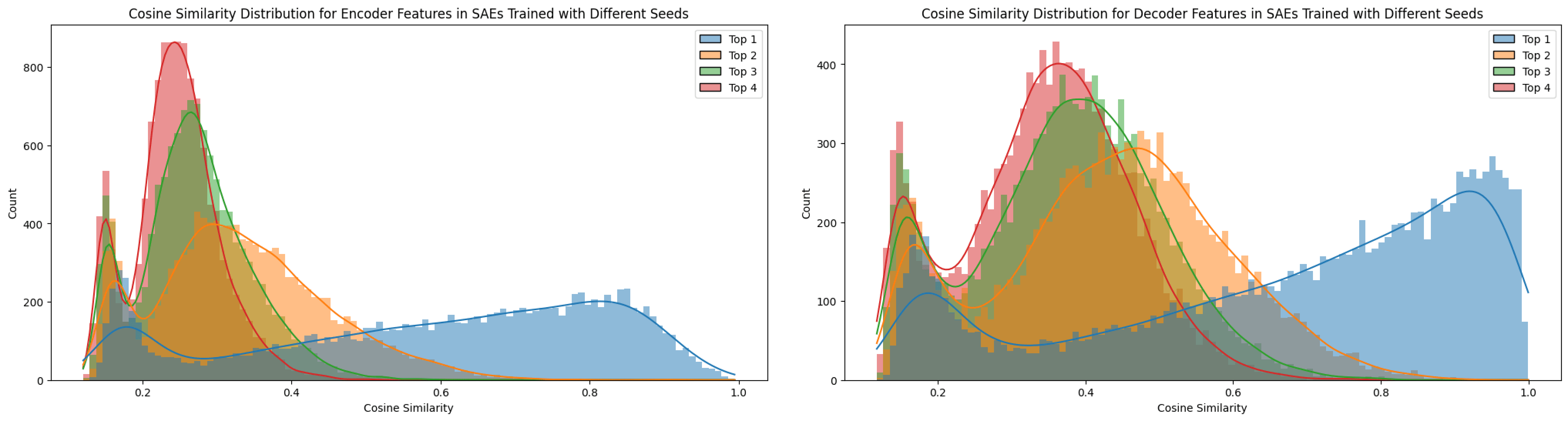
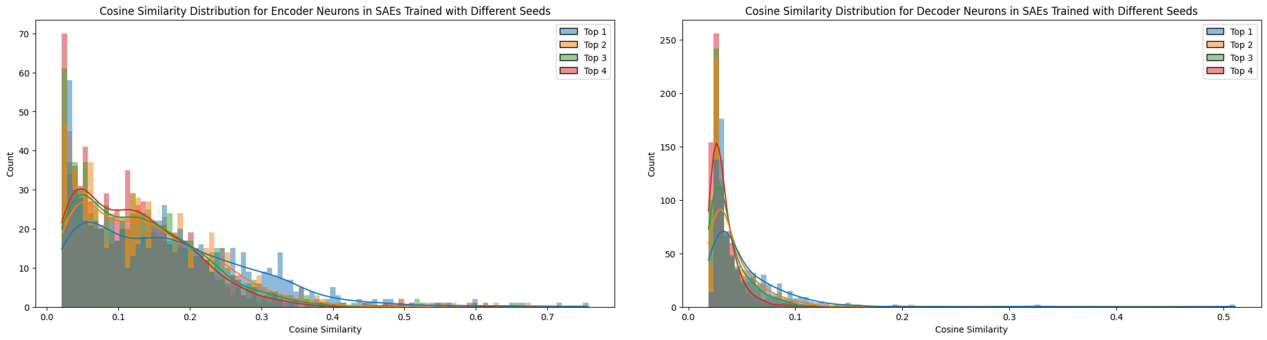
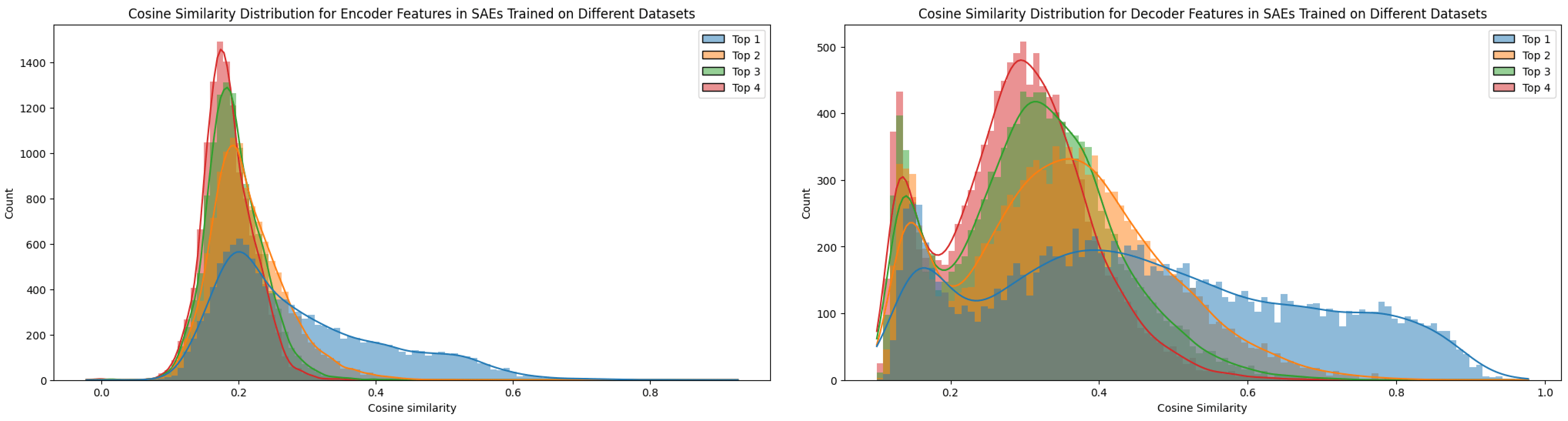
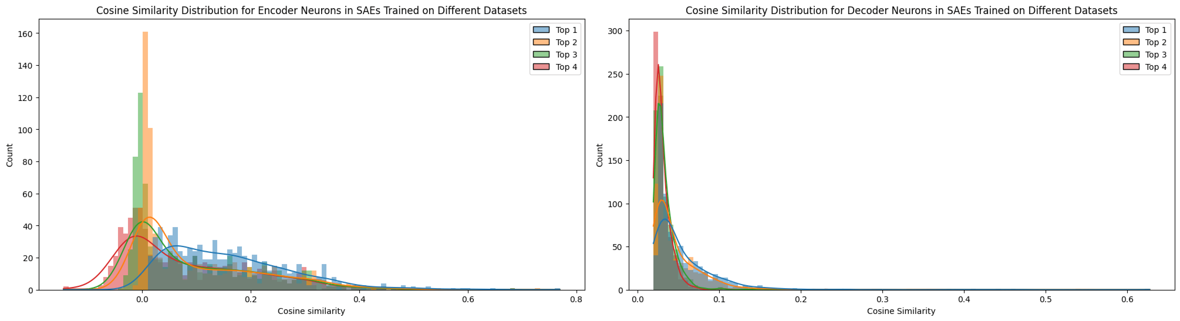
The top-1 cosine similarity for features across SAEs trained with different seeds exhibited many significantly high values (see Figure 11). However, not every feature proved universal, as the top‑n cosine similarities remained relatively elevated, suggesting the presence of superpositioned features. In contrast, when training on different datasets (e.g., TinyStories versus OpenWebText), the feature similarity dropped compared to the seed-only test. This comparison will be discussed in further detail in the next section.

Notably, the matching ratios differ considerably between the encoder and decoder methods, a pattern that held true across all matching experiments. The higher matching ratio from the decoder and the higher neuron matching from the encoder suggest distinct roles for these matrices. Conceptually, as noted by Nanda (2023) [AF · GW], the encoder and decoder perform different functions. In my interpretation, based on Figures 3 and 4, the decoder weights are directly influenced by the L2 reconstruction loss, which encourages them to exploit features as fully as possible. This allows the decoder to freely represent feature directions without the same sparsity pressure (Nanda, 2023 [AF · GW]). In contrast, the encoder weights, being subject to an L1 sparsity loss on the feature vector, are constrained in their ability to represent features, effectively “shrinking” their representation capacity as Figure 3. Thus, the encoder focuses more on detect sparse features by disentangling superpositioned features under sparsity constraints (Nanda, 2023 [AF · GW]).

A similar rationale applies to neuron similarity in each weight matrix. It is interesting to note that the patterns for encoder and decoder differ markedly. As explained in Figures 3 and 4, the overall lower cosine similarity for neurons may be attributed to the high dimensionality of the neuron weight vectors (e.g., a dictionary size of 12,288), which makes it less likely for their directions to align due to the curse of dimensionality. Although lowering the threshold could force more matches, doing so would not yield consistent results across the same model. For this reason, I have compared the influences of different SAE training factors with tool of decoder-based feature matching.

4.2.2 Effect of Training Settings on Feature Matching

The following tables summarize how various training factors affect the feature matching ratio.

Dataset Difference
TinyStories vs. RedPajama	TinyStories vs. Pile	OpenWebText vs. TinyStories	OpenWebText vs. RedPajama	Pile vs. RedPajama
6.21%	11.48%	15.45%	23.56%	29.48%

Dictionary Difference (OpenWebText / TinyStories)
12288 in 3072	12288 in 6144	6144 in 3072
25.56% / 22.27%	39.36% / 40.62%	47.15% / 43.47%

Dictionary Difference (OpenWebText / TinyStories)
6144 in 12288	3072 in 12288	3072 in 6144
72.77% / 77.25%	89.22% / 78.16%	89.25% / 80.01%

Seed 42 vs. Seed 49 (OpenWebText / TinyStories)
Dictionary 12288	Dictionary 6144	Dictionary 3072
54.85% / 55.65%	65.90% / 71.37%	83.46% / 71.37%

Architecture Difference (OpenWebText / TinyStories)
Top-k vs. BatchTopK	JumpReLU vs. BatchTopK	Top-k vs. JumpReLU
53.94% / 42.80%	60.20% / 45.36%	56.56% / 42.80%

Sparsity Difference (OpenWebText / TinyStories)
Top-k 16 vs. Top-k 64	Top-k 32 vs. Top-k 64	Top-k 16 vs. Top-k 32
42.83% / 33.06%	55.51% / 42.96%	54.95% / 49.60%

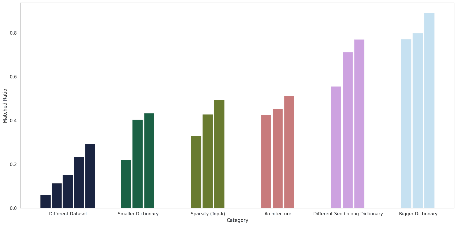
Table 1. I trained SAEs with modifications in six categories and compared the resulting feature matching ratios using a threshold of ${\tau }_{feature}=0.7$. For the seed comparison, I focused on changes driven by dictionary size variations, as comparing multiple seeds directly would be less informative.

Examining these results, several insights emerge. First, when all other settings are held constant and only the dictionary size is varied, a large proportion of the features in the smaller dictionary are present in the larger one, as expected. Moreover, while architecture and sparsity do affect the matching ratio, their impact is not as pronounced as that of the dataset.

Key observations from the experiments include:

1. Dataset: The characteristics of the dataset clearly affect the matching ratio. For example, the synthetic TinyStories data exhibited a lower matching ratio compared to the web-crawled datasets. When testing on OpenWebText and TinyStories under the same experimental conditions, TinyStories, despite its presumed lower diversity, yielded a lower feature matching ratio.^[4]
2. Seed Difference: The matching ratios between different seeds were relatively high (ranging from 55% to 85%), which is notably higher than the approximately 30% reported in Paulo & Belrose (2025). I discuss this discrepancy further below.
3. Feature Sparsity: Reducing sparsity led to a decrease in the feature matching ratio, which ranged between 40% and 55%, with no clear regular pattern emerging.
4. Dictionary Size Difference: When comparing dictionaries of different sizes, features from the smaller dictionary were often contained within the larger one. As shown in Table 2, the difference in the number of matched features relative to the overall dictionary size was modest, supporting the choice of the threshold ${\tau }_{feature}$.
5. Architecture Difference: Overall, the results here were inconsistent. Although I initially expected that similar activation functions (e.g., Top‑k versus BatchTopK) would yield higher matching ratios, the results hovered between 40% and 60% without a clear trend.

	3072 vs. 12288	6144 vs 12288	3072 vs 6144
OpenWebText	400	366	156
TinyStories	332	251	212

Table 2. Feature count difference (calculated as larger dictionary feature count minus the smaller dictionary’s feature count $\text{Dictionary size}\times \text{Feature Matching ratio}$, weighted by the feature matching ratio). The horizontal axis represents the dictionary size comparisons, and the vertical axis corresponds to the two datasets.

I initially had a hypothesis regarding seed differences. My position aligns with the statement from Bricken et al. (2023) optimistically: "We conjecture that there is some idealized set of features that dictionary learning would return if we provided it with an unlimited dictionary size." The idea is that this idealized set may be quite large, and that the variations I see are due to weight initialization and the use of a dictionary size smaller than ideal. Consequently, my alternative hypothesis was that increasing the dictionary size would lead to a higher feature matching ratio.

However, after the experiment, the common feature ratio decreased drastically as Paulo & Belrose, 2025 shown. this finding challenges the initial hypothesis, and I suspect this is because the reconstruction pressure varies with dictionary size, thereby changing the abstraction level of the features. As Bricken et al. noted, changes in dictionary size can lead to feature splitting (Chanin et al., 2024), where context features break down into token-in-context features, splitting into a range of granular possibilities. In this scenario, instead of converging on a fixed set of optimal features, the features adapt to different abstraction levels depending on the dictionary size, resulting in a higher probability of common feature combinations at lower dictionary sizes.

For future interpretability, I see a need for approaches that can simultaneously discover multi-level features, such as the Matryoshka SAE (Nabeshima, 2025 [LW · GW]; Bussmann, 2025 [LW · GW]), while still acknowledging the possibility of superposition and identifying specific robust features that remain consistent regardless of dictionary size.

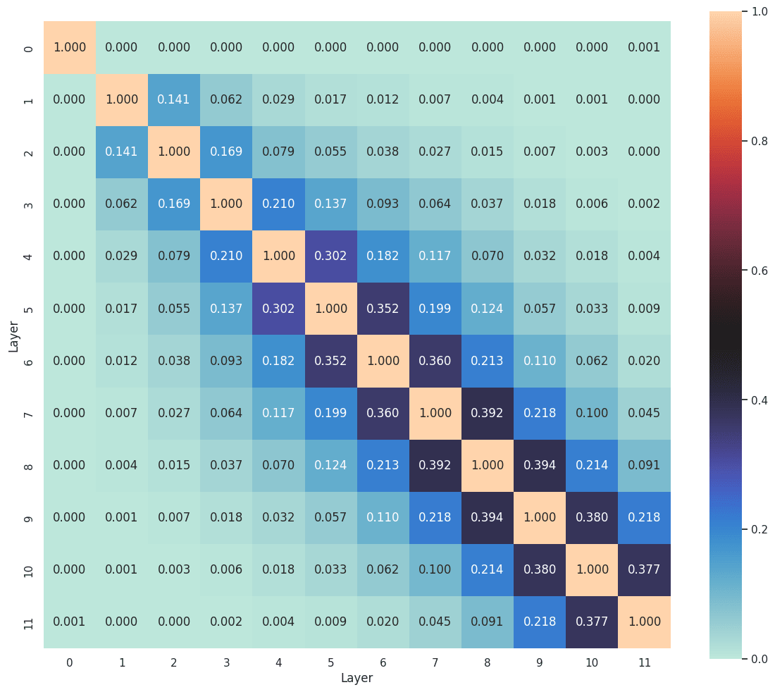
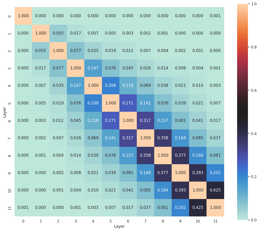
4.2.3 Feature Matching along the layers

It is well established that adjacent layers in a transformer tend to share more features (Ghilardi et al., 2024; Dunefsky & Chlenski, 2024; Lindsey et al., 2024). Features often evolve, disappear, or merge as one moves through the layers. A low matching ratio between adjacent layers suggests that the feature sets have already diverged. In Figure 12, the early layers exhibit considerably lower feature matching between each other, a trend that mirrors the cosine similarity patterns observed in Lindsey et al. (2024). This phenomenon provides tentative support for the idea that certain features, such as the position features suggested in Section 4.1.2, vanish rapidly in the early stages of the network.

5. Conclusion

In this work, I proposed that the dataset is the factor that most strongly influences changes in the dictionary (total feature set) during dictionary learning. Additionally, by analyzing feature activation distributions across positions, I hypothesize that a distinct position-related feature set emerges in the early layers. I explored two interconnected aspects: activation distributions and feature transferability. Specifically, the dataset affects feature matching more than differences in initialization seeds, while variations in sparsity and architecture also alter the feature set, albeit to a lesser extent. Dictionary size plays a complex role, as it influences the abstraction level of the overall features. Moreover, the low feature matching observed between early layers, combined with the doubling of the activation frequency along token positions and the visually distinct separation of the feature set, supports the existence of a position feature set in the initial layers.

6. Limitation

First of all, the experiments are limited to GPT2-small, meaning that the lack of model diversity restricts the generalization of the claims across different models. Furthermore, the logical sequence underpinning the claim of a position feature set in Section 4.2, derived from token position and early layers, contains certain leaps. One alternative explanation is that the single-token feature set in the early layer is due to token embeddings. Additionally, not training the SAE on the full token sequence, coupled with the observed increase in cross-entropy after reconstruction and the application of positional zero clamping and feature shuffling under severe performance degradation, which presupposes that the feature set remains reflective of the underlying structure.

Moreover, feature matching here did not apply a geometric median (Bricken et al., 2023; Gao et al., 2024), to all SAE trainings. Although a geometric median-based weight initialization might enhance robustness with respect to seed or dataset differences, I did not compare this approach. Finally, as noted above, not applying the Hungarian algorithm may have led us to overestimate the similarity, producing slightly optimistic numbers that are not strictly comparable with previous studies.

7. Future works

Based on my observations from token positions and early layers, I formulated a multi-step hypothesis (steps 1-4 in Section 4.2). If these steps and their causal relationships can be validated, it could provide an intriguing perspective on how transformers interpret position through monosemantic features. Furthermore, to improve feature matching, applying a geometric median (as per Bricken et al. (2023) and Gao et al. (2024)) might increase the matching ratio and shed light on the influence of dataset dependency, for instance, how geometric median-based weight initialization affects feature matching across different seeds and datasets. In this study, I primarily examined feature matching ratios rather than interpretability scores. Future work could explore how training settings affect Automated Interpretability Score (Bills et al., 2023) or Eluether embedding (Paulo et al., 2024).

8. Acknowledgments

This research was conducted using the resources of the UCL Computing Lab. I am grateful to the supportive community on LessWrong for their insightful contributions. Special thanks to @Joseph Bloom [LW · GW] @chanind [LW · GW] for providing the open-source SAE Lens, and to @Neel Nanda [LW · GW] for the Transformer Lens that formed the basis of much of this work. I also thank @Bart Bussmann [LW · GW] for publishing the BatchTopK source code, which was both minimal and reproducible. Finally, I appreciate the diverse discussions with my UCL colleagues that helped me uncover valuable sources on SAEs.

9. Appendix

9.1. Implementation Details

All source code for running the scripts is available here, and the proof-of-concept notebooks can be found here.

9.2. Activation Average versus Standard Deviation

9.4. LLM Loss and SAE Loss

9.5 UMAPs of feature directions

9.6. Trained SAEs options

Architecture	Seed	Dictionary	Dataset	Sparsity (k/ L1 coeff)	Layer
Top-k	42/49	768×4/8/16	OpenWebText	16/32/64	8
Top-k	42/49	768×4/8/16	TinyStories	16/32/64	8
Top-k	49	768×16	RedPajama	16	8
Top-k	49	768×16	Pile Uncopyrighted	16	8
Top-k	49	768×16	TinyStories	16/32	0-11
BatchTopK	49	768×16	OpenWebText	16/32/64	8
BatchTopK	42/49	768×16	TinyStories	16/32/64	8
JumpReLU	49	768×16	TinyStories	0.004/0.0018/0.0008	8

Table 3. A total of 73 SAEs were trained; all hyperparameters not specified here are the same as in the baseline setting.^[5]

1. ^{^}

   I disregarded the shared pre-bias for centering inputs and outputs, which is commonly used.

2. ^{^}

   The BOS token was always set as the first token, as Tdooms & Danwil (2024) noted that this maintains model performance, which is consistent with my empirical observations and for simplicity.

3. ^{^}

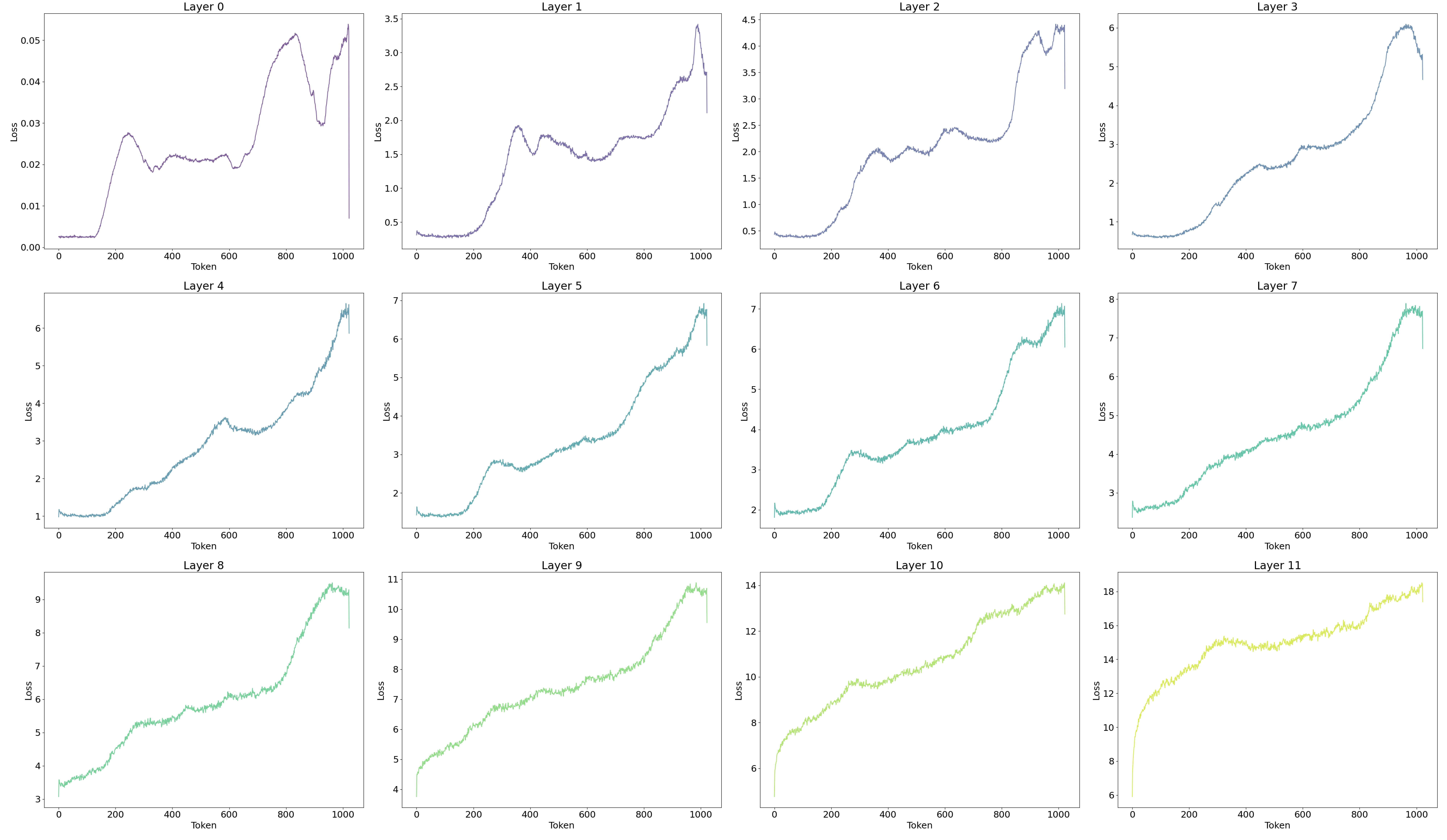
   According to Heimersheim & Turner, 2023 [AF · GW], residual stream norms grow exponentially over the forward pass, which may contribute to increasing reconstruction loss along the layers.

4. ^{^}

   I excluded the OpenWebText and The Pile comparison in the experiment since OpenWebText is a subset of The Pile.

5. ^{^}

   The baseline setting is a layer 8 Top‑k Z-model with Top‑k 16, using the OpenWebText dataset, a sequence length of 128, a learning rate of 0.0003, and a seed 49

Additional Comments

This is my very first posting on LessWrong. I have read many fascinating articles in this field, and I am excited to share my first post. I plan to continue pursuing research on improving the SAE architecture, efficient steering, and transferability. I welcome any advice or corrections. Please feel free to provide feedback on my first post.

0 comments

Comments sorted by top scores.