The Lightcone Theorem: A Better Foundation For Natural Abstraction?

post by johnswentworth · 2023-05-15T02:24:02.038Z · LW · GW · 25 comments

Contents

  The Proof, In Pictures
  How To Use The Lightcone Theorem?
None
25 comments

Thankyou to David Lorell for his contributions as the ideas in this post were developed.

For about a year and a half now, my main foundation for natural abstraction math has been The Telephone Theorem [LW · GW]: long-range interactions in a probabilistic graphical model (in the long-range limit) are mediated by quantities which are conserved (in the long-range limit). From there, the next big conceptual step [LW · GW] is to argue that the quantities conserved in the long-range limit are also conserved by resampling, and therefore the conserved quantities of an MCMC sampling process on the model mediate all long-range interactions in the model.

The most immediate shortcoming of the Telephone Theorem and the resampling argument is that they talk about behavior in infinite limits. To use them, either we need to have an infinitely large graphical model, or we need to take an approximation. For practical purposes, approximation is clearly the way to go, but just directly adding epsilons and deltas to the arguments gives relatively weak results.

This post presents a different path.

The core result is the Lightcone Theorem:

• Start with a probabilistic graphical model on the variables $X_1,\dots ,X_n$.
  • The graph defines adjacency, distance, etc between variables. For directed graphical models (i.e. Bayes nets), spouses (as well as parents and children) count as adjacent.
• We can model those variables as the output of a Gibbs sampler (that’s the MCMC process) on the graphical model.
  • Call the initial condition of the sampler $X^0=(X_1^0,\dots ,X_n^0)$. The distribution of $X^0$ must be the same as the distribution of $X$ (i.e. the sampler is initialized “in equilibrium”).
  • We can model the sampler as having run for any number of steps to generate the variables; call the number of steps $T$.
  • At each step, the process resamples some set of nonadjacent variables conditional on their neighbors.
• The Lightcone Theorem says: conditional on $X^0$, any sets of variables in $X$ which are a distance of at least $2T$ apart in the graphical model are independent.
  • Yes, exactly independent, no approximation.

In short: the initial condition of the resampling process provides a latent, conditional on which we have exact independence at a distance.

This was… rather surprising to me. If you’d floated the Lightcone Theorem as a conjecture a year ago, I’d have said it would probably work as an approximation for large $T$, but no way it would work exactly for finite $T$. Yet here we are.

The Proof, In Pictures

The proof is best presented visually.^[1] High-level outline:

• Perform a do() operation on the Gibbs sampler, so that it never resamples the variables a distance of $T$ from $X_R$.
• In the do()-operated process, $X^0$ mediates between $X_R^T$ and $X_{D(R,\ge 2T)}^T$, where $D(R,\ge 2T)$ indicates indices of variables a distance of at least $2T$ from $X_R$.
• Since $X^0$, $X_R^T$ and $X_{D(R,\ge 2T)}^T$ are all outside the lightcone of the do()-operation, they have the same joint distribution under the non-do()-operated sampler as under the do()-operated sampler.
• Therefore $X^0$ mediates between $X_R^T$ and $X_{D(R,\ge 2T)}^T$ under the original sampler.

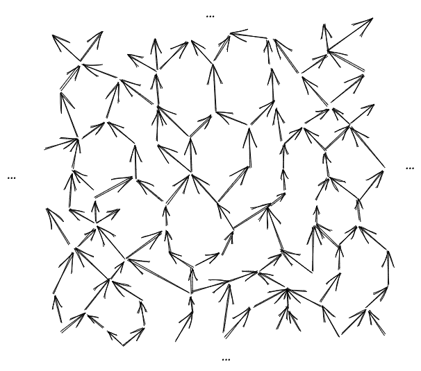
We start with the graphical model:

Within that graphical model, we’ll pick some tuple of variables $X_R$ (“R” for “region”)^[2]. I’ll use the notation $X_{D(R,t)}$ for the variables a distance $t$ away from $R$, $X_{D(R,>t)}$ for variables a distance greater than $t$ away from $R$, $X_{D(R,<t)}$ for variables a distance less than $t$ away from $R$, etc.

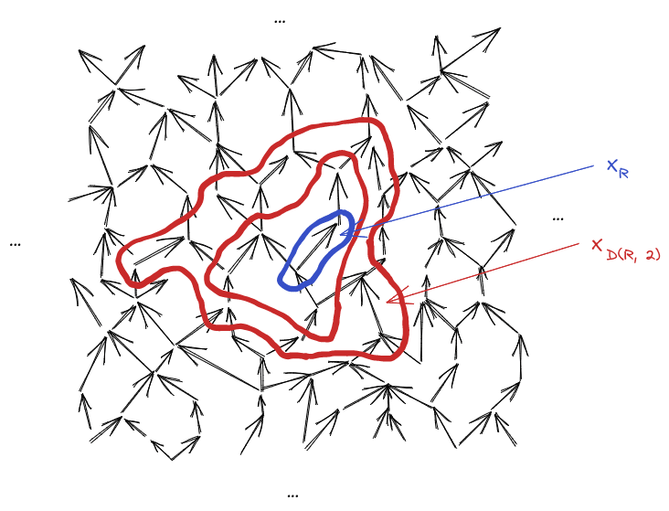
Note that for any $t$, $X_{D(R,t)}$ (the variables a distance $t$ away from $R$) is a Markov blanket, mediating interaction between $X_{D(R,<t)}$ (everything less than distance $t$ from $X_R$), and $X_{D(R,>t)}$ (everything more than distance $t$ from $X_R$).

Next, we’ll draw the Gibbs resampler as a graphical model. We’ll draw the full state $X^t$ at each timestep as a “layer”, with $X^0$ as the initial layer and $X=X^T$ as the final layer. At each timestep, some (nonadjacent) variables are resampled conditional on their neighbors, so we have arrows from the neighbor-variables in the previous timestep. The rest of the variables stay the same, so they each just have a single incoming variable from themselves at the previous timestep.

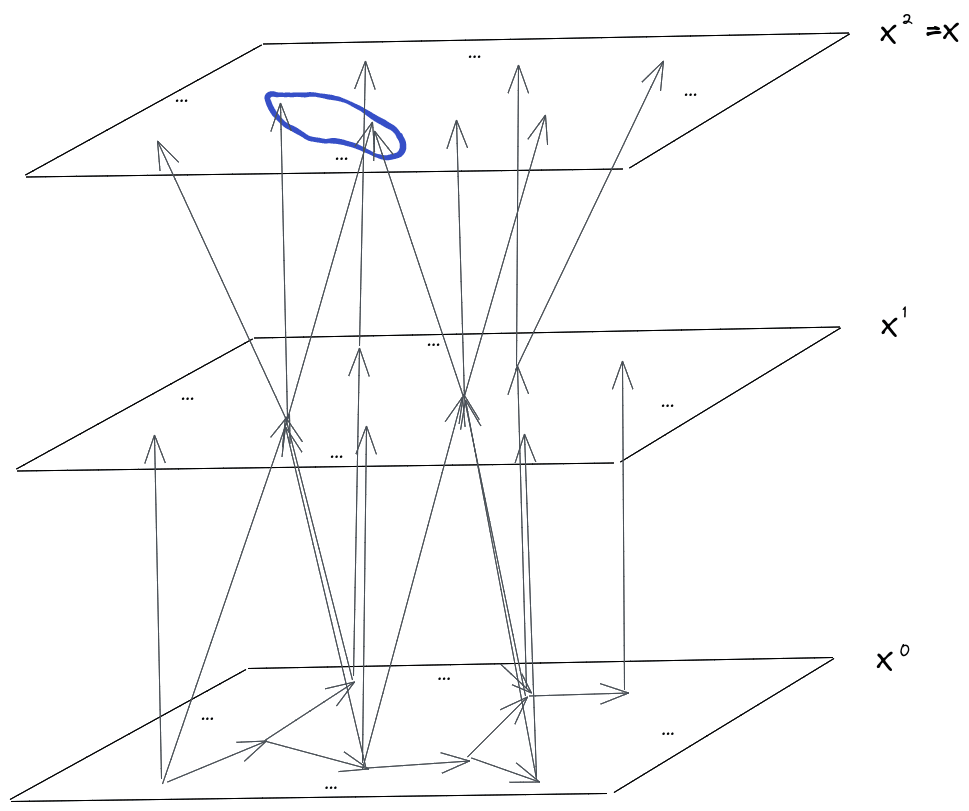
Now for the core idea: we’re going to perform a do() operation on the resampler-graph. Specifically, we’re going to hold $X_{D(R,T)}$ constant; none of the variables in that Markov blanket are ever resampled in the do()-transformed resampling process.

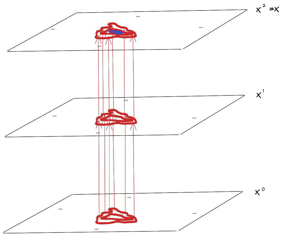
Notice that, in the do()-operated process, knowing $X^0$ also tells us the value of $X_{D(R,T)}^t$ for all $t$. So, if we condition on $X^0$, then visually we’re conditioning on:

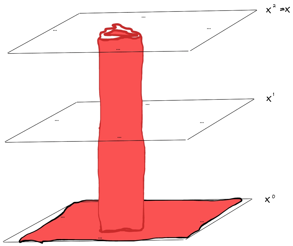
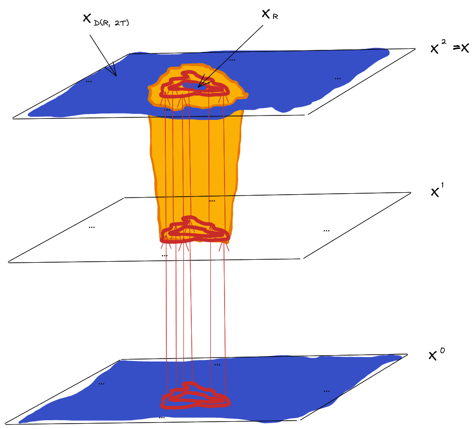
Note that the “cylinder” (including the “base”) separates $X^T$ into two pieces - one contains everything less than distance $T$ from $X_R^1,...,X_R^T$, and the other everything more than distance $T$ from $X_R^1,...,X_R^T$. The separation indicates that $X^0$ is a Markov blanket between those pieces… at least within the do()-operated resampling process.

Now for the last step: we’ll draw a forward “lightcone” around our do()-operation. As the name suggests, it expands outward along outgoing arrows, starting from the nodes intervened-upon, to include everything downstream of the do()-intervention.

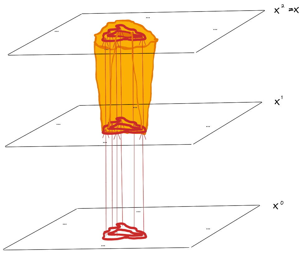
Outside of that lightcone, the distribution of the do()-operated process matches that of the non-do()-operated process.

Crucially, $X^0$, $X_R^T=X_R$, and $X_{D(R,\ge 2T)}^T=X_{D(R,\ge 2T)}$ are all outside of the lightcone, so their joint distribution is the same under the do()-operated and non-do()-operated resampling process.

Since $X^0$ mediates between $X_R$ and $X_{D(R,\ge 2T)}^T$ in the do()-operated process, and the joint distribution is the same between the do()-operated and non-do()-operated process, $X^0$ must mediate between $X_R$ and $X_{D(R,\ge 2T)}^T$ under the non-do()-operated process.

In other words: any two sets of variables at least a distance of $2T$ apart (i.e. $X_R$ and $X_{D(R,\ge 2T)}^T$) are independent given $X^0$. That’s the Lightcone Theorem for two sets of variables.

Finally, note that we can further pick out two subsets of $X_{D(R,\ge 2T)}^T$ which are themselves separated by $2T$, and apply the Lightcone Theorem for two sets of variables again to conclude that $X_R$ and the two chosen sets of variables are all mutually independent given $X^0$. By further iteration, we can conclude that any number of sets of variables which are all separated by a distance of $2T$ are independent given $X^0$. That’s the full Lightcone Theorem.

How To Use The Lightcone Theorem?

The rest of this post is more speculative.

$X^0$ mediates interactions in $X$ over distance of at least $2T$, but $X^0$ also typically has a bunch of “extra” information in it that we don’t really care about - information which is lost during the resampling process. So, the next step is to define the latent $\Lambda$:

$\Lambda \left(X^0\right):=(x\mapsto lnP[X=x|X^0\left]\right)$

By the minimal map [LW · GW] argument, $\Lambda =P\left[X|\Lambda \right]=P\left[X|X^0\right]$; $\Lambda$ is an informationally-minimal summary of all the information in $X^0$ relevant to $X$.

… but that doesn’t mean that $\Lambda$ is minimal among approximate summaries, nor that it’s a very efficient representation of the information. Those are the two main open threads: approximation and efficient representation.

On the approximation front, a natural starting point is to look at the eigendecomposition of the transition matrix for the resampling process. This works great in some ways, but plays terribly with information-theoretic quantities (logs blow up for near-zero probabilities). An eigendecomposition of the log transition probabilities plays better information-theoretic quantities, but worse with composition as we increase $T$, and we’re still working on theorems to fully justify the use of the log eigendecomposition.

On the efficient representation front, a natural stat-mech-style starting point is to pick “mesoscale regions”: $m$ sets of variables $X_{R_1},...,X_{R_m}$ which are all separated by at least distance $2T$, but big enough to contain the large majority of variables. Then

$lnP[X_{R_1},\dots ,X_{R_m}|\Lambda ]={\sum }_{i}lnP\left[X_{R_i}|\Lambda \right]$

At this point the physicists wave their hands REALLY vigorously and say “... and since $X_{R_1},...,X_{R_m}$ includes the large majority of variables, that sum will approximate $P\left[X|\Lambda \right]$”. Which is of course extremely sketchy, but for some (very loose) notions of “approximate” it can work for some use cases. I’m still in the process of understanding exactly how far that kind of approximation can get us, and for what use-cases.

Insofar as the mesoscale approximation does work, another natural step is to invoke generalized Koopman-Pitman-Darmois [LW · GW] (gKPD). This requires a little bit of a trick: a Gibbs sampler run backwards is still a Gibbs sampler. So, we can swap $X^0$ and $X$ in the Lightcone Theorem: subsets of $X^0$ separated by a distance of at least $2T$ are independent given $X$. From there:

• $\Lambda \left(X^0\right)$ is a summary of all information in $X^0$ relevant to $X$
• Insofar as the mesoscale argument works, “most of” $X^0$ is independent given $X$

… which is most of what we need to apply gKPD. If we ignore the sketchy part - i.e. pretend that regions $X_{R_1}^0,...,X_{R_m}^0$ cover all of $X^0$ and are all independent given $X$ - then gKPD would say roughly: if $\Lambda$ can be represented as $n/2$ dimensional or smaller, then $\Lambda$ is isomorphic to ${\sum }_i{f}_i\left(X_{R_i}\right)$ for some functions $f_i$, plus a limited number of “exception” terms. There’s a lot of handwaving there, but that’s very roughly the sort of argument I hope works. If successful, it would imply a nice maxent form (though not as nice as the maxent form I was hoping for [LW · GW] a year ago, which I don’t think actually works), and would justify using an eigendecomposition of the log transition matrix for approximation.

1. ^{^}

   I’ve omitted from the post various standard things about Gibbs samplers, e.g. explaining why we can model the variables of the graphical model as the output of a Gibbs sampler, how big $T$ needs to be in order to resample all the variables at least once, how to generate $X^0$ from $X$ (rather than vice-versa), etc. Leave a question in the comments if you need more detail on that.

2. ^{^}

   Notation convention: capital-letter indices like $X_A$ indicate index-tuples, i.e. if $A=(1,2,3)$ then $X_A=(X_1,X_2,X_3)$.

25 comments

Comments sorted by top scores.