How long does it take to become Gaussian?
post by Maxwell Peterson (maxwell-peterson) · 2020-12-08T07:23:41.725Z · LW · GW · 40 commentsContents
  Identically-distributed distributions converge quickly
  An easier way to measure Gaussianness (Gaussianity?)
  Non-identically-distributed distributions converge quickly too
None
40 comments
The central limit theorems all say that if you convolve stuff enough, and that stuff is sufficiently nice, the result will be a Gaussian distribution. How much is enough, and how nice is sufficient?
Identically-distributed distributions converge quickly
For many distributions , the repeated convolution looks Gaussian. The number of convolutions you need to look Gaussian depends on the shape of . This is the easiest variant of the central limit theorem: identically-distributed distributions.
The uniform distribution converges real quick:
The numbers on the x axis are increasing because the mean of is the sum of the means [? · GW] of and , so if we start with positive means, repeated convolutions shoot off into higher numbers. Similar for the variance - notice how the width starts as the difference between 1 and 2, but ends with differences in the tens. You can keep the location stationary under convolution by starting with a distribution centered at 0, but you can't keep the variance from increasing, because you can't have a variance of 0 (except in the limiting case).
Here's a more skewed distribution: beta(50, 1). beta(50, 1) is the probability distribution that represents knowing that a lake has bass and carp, but not how many of each, and then catching 49 bass in a row. It's fairly skewed! This time, after 30 convolutions, we're not quite Gaussian - the skew is still hanging around. But for a lot of real applications, I'd call the result "Gaussian enough".
A similar skew in the opposite direction, from the exponential distribution:
I was surprised to see the exponential distribution go into a Gaussian, because Wikipedia says that an exponential distribution with parameter goes into a gamma distribution with parameters gamma(, ) when you convolve it with itself times. But it turns out gamma() looks more and more Gaussian as goes up.
How about our ugly bimodal-uniform distribution?
It starts out rough and jagged, but already by 30 convolutions it's Gaussian.
And here's what it looks like to start with a Gaussian:
The red curve starts out the exact same as the black curve, then nothing happens because Gaussians stay Gaussian under self-convolution.
An easier way to measure Gaussianness (Gaussianity?)
We're going to want to look at many more distributions under convolutions and see how close they are to Gaussian, and these animations take a lot of space. We need a more compact way. So let's measure the kurtosis of the distributions, instead. The kurtosis is the fourth moment of a probability distribution; it describes the shape of the tails. All Gaussian distributions have kurtosis 3. There are other distributions with kurtosis 3, too, but they're not likely to be the result of a series of convolutions. So to check how close a distribution is to Gaussian, we can just check how far from 3 its kurtosis is.
We can chart the kurtosis as a function of how many convolutions have been done so far, for each of the five distributions above:
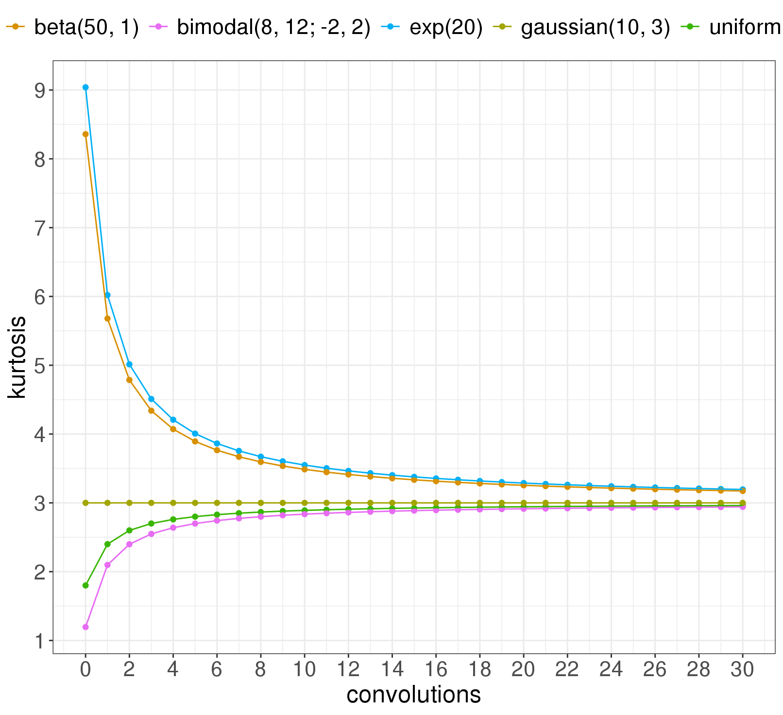
Notice: the distributions that have a harder time making it to Gaussian are the two skewed ones. It turns out the skew of a distribution goes a long way in determining how many convolutions you need to get Gaussian. Plotting the kurtosis at convolution 30 against the skew of the original distribution (before any convolutions) shows that skew matters a lot:
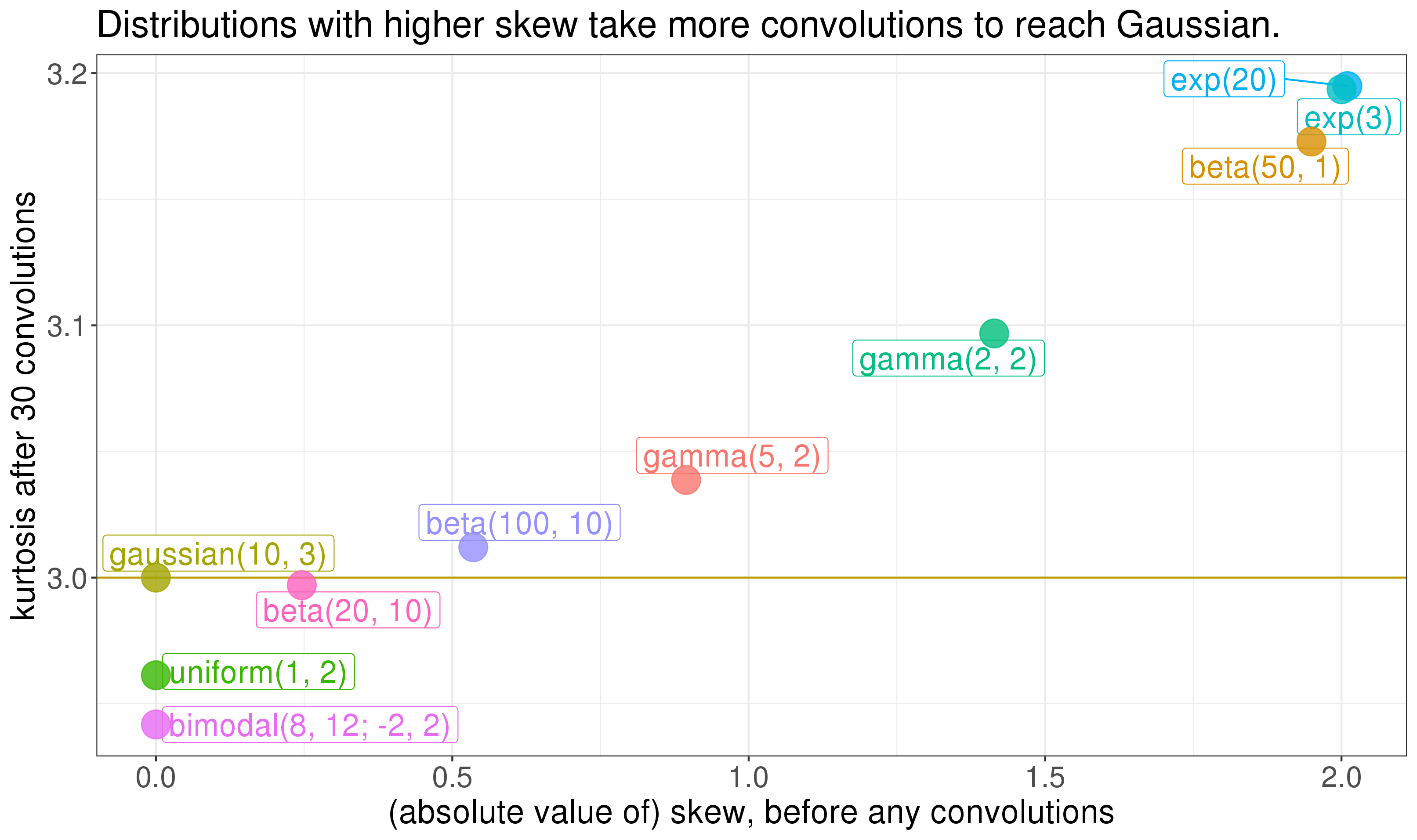
So the skew of the component distributions goes a long way in determining how quick their convolution gets Gaussian. The Berry-Esseen theorem is a central limit theorem that says something similar (but see this comment [LW(p) · GW(p)]). So here's our first rule for eyeing things in the wild and trying to figure out whether the central limit theorem will apply well enough to get you a Gaussian distribution: how skewed are the input distributions? If they're viciously skewed, you should worry.
Non-identically-distributed distributions converge quickly too
In real problems, distributions won't be identically distributed. This is the interesting case. If instead of a single distribution convolved with itself, we take , then a version of the central limit theorem still applies - the result can still be Gaussian. So let's take a look.
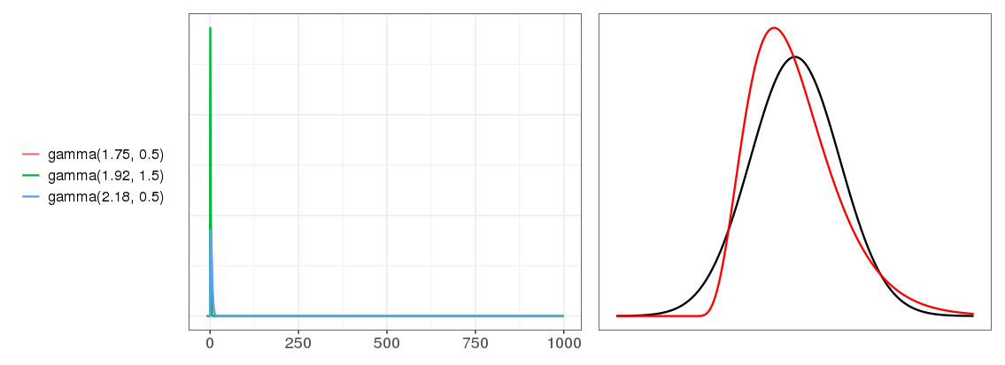
Here are three different Beta distributions, on the left, and on the right, their convolution, with same setup from the animations: red is the convolution, and black is the true Gaussian with the same mean and variance.
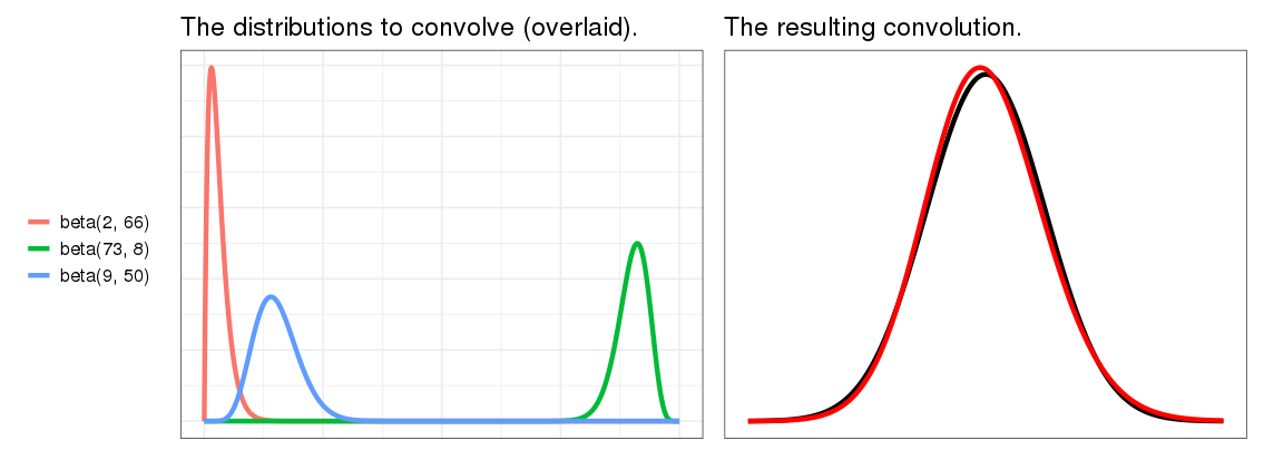
They've almost converged! This is a surprise. I really didn't expect as few as three distributions to convolve into this much of a Gaussian. On the other hand, these are pretty nice distributions - the blue and green look pretty Gaussian already. That's cheating. Let's try less nice distributions. We saw above that distributions with higher skew are less Gaussian after convolution, so let's crank up the skew. It's hard to get a good skewed Beta distribution, so let's use Gamma distributions instead.
Not Gaussian yet - the red convolution result line still looks Gamma-ish. But if we go up to a convolution of 30 gamma distributions this skewed...
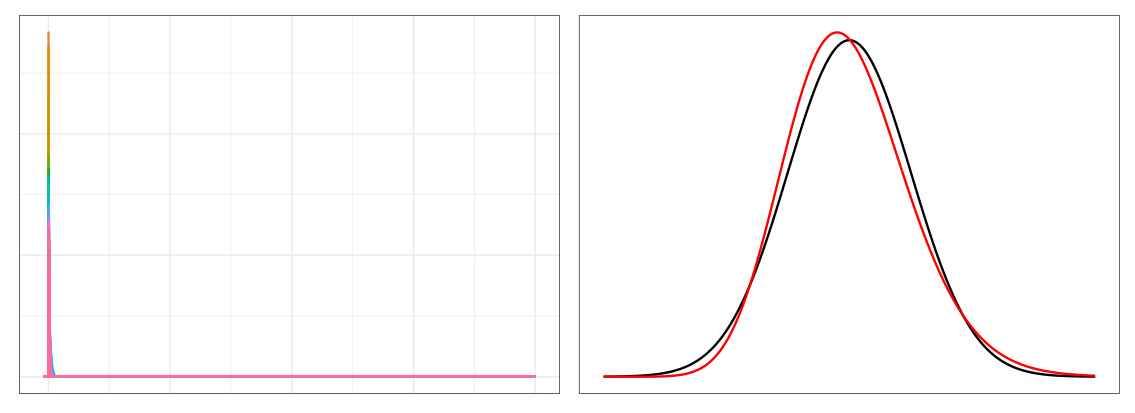
... already, we're pretty much Gaussian.
I'm really surprised by this. I started researching this expecting the central limit theorem convergence to fall apart, and require a lot of distributions, when the input distributions got this skewed. I would have guessed you needed to convolve hundreds to approach Gaussian. But at 30, they're already there! This helps explain how carefree people can be in assuming the CLT applies, sometimes even when they haven't looked at the distributions: convergence really doesn't take much.
40 comments
Comments sorted by top scores.
comment by Donald Hobson (donald-hobson) · 2020-12-08T10:23:23.574Z · LW(p) · GW(p)
All Gaussian distributions have kurtosis 3, and no other distributions have kurtosis 3. So to check how close a distribution is to Gaussian, we can just check how far from 3 its kurtosis is.
This is wrong. kurtosis is just the expectation of the 4th power. (Edit: renormalized by expectations of the first and second power) All sorts of distributions have kurtosis 3. Like for example the discrete distribution over [-1,0,0,0,0,1]
Otherwise an interesting post.
Replies from: Gunnar_Zarncke, maxwell-peterson↑ comment by Gunnar_Zarncke · 2020-12-08T14:56:10.063Z · LW(p) · GW(p)
I'm not sure Kurtosis is the right measure for how Gaussian is in practice. I would have been more interested in the absolute difference between the distributions. That might be more difficult to compute though.
Replies from: climbert8, Bucky, maxwell-peterson↑ comment by climbert8 · 2020-12-09T09:37:04.441Z · LW(p) · GW(p)
To that point, skew and excess Kurtosis are just two of an infinite number of moments, so obviously they do not characterize the distribution. As someone else here suggested, one can look at the Fourier (or other) Transform, but then you are again left with evaluating the difference between two functions or distributions: knowing that the FT of a Gaussian is a Gaussian in its dual space doesn't help with "how close" a t-domain distribution F(t) is to a t-domain Gaussian G(t), you've just moved the problem into dual space.
We have a tendency to want to reduce an infinite dimensional question to a one dimensional answer. How about the L1 norm or the L2 norm of the difference? Well, the L2 norm is preserved under FT, so nothing is gained. Using the L1 norm would require some justification other than "it makes calculation easy".
So it really boils down to what question you are asking, what difference does the difference (between some function and the Gaussian) make? If being wrong (F(t) != G(t) for some t) leads to a loss of money, then use this as the "loss" function. If it is lives saved or lost use that loss function on the space of distributions. All such loss functions will look like an integral over the domain of L(F(t), G(t)). In this framework, there is no universal answer, but once you've decided what your loss function is and what your tolerance is you can now compute how many approximations it takes to get your loss below your tolerance.
Another way of looking at it is to understand what we are trying to compare the closeness of the test distribution to. It is not enough to say F(t) is this close to the Gaussian unless you can also tell me what it is not. (This is the "define a cat" problem for elementary school kids.) Is it not close to a Laplace distribution? How far away from Laplace is your test distribution compared to how far away it is from Gaussian? For these kinds of questions - where you want to distinguish between two (or more) possible candidate distributions - the Likelihood ratio is a useful metric.
Most data sceancetists and machine learning smiths I've worked with assume that in "big data" everything is going to be a normal distribution "because Central Limit Theorem". But they don't stop to check that their final distribution is actually Gaussian (they just calculate the mean and the variance and make all sorts of parametric assumptions and p-value type interpretations based on some z-score), much less whether the process that is supposed to give rise to the final distribution is one of sampling repeatedly from different distributions or can be genuinely modeled as convolutions.
One example: the distribution of coefficients in a Logistic model is assumed (by all I've spoken to) to be Gaussian ("It is peaked in the middle and tails off to the ends."). Analysis shows it to be closer to Laplace, and one can model the regression process itself as a diffusion equation in one dimension, whose solution is ... Laplace!
I can provide an additional example, this time of a sampling process, where one is sampling from hundreds of distributions of different sizes (or weights), most of which are close to Gaussian. The distribution of the sum is once again, Laplace! With the right assumptions, one can mathematically show how you get Laplace from Gaussians.
Replies from: Gunnar_Zarncke↑ comment by Gunnar_Zarncke · 2020-12-09T15:26:26.543Z · LW(p) · GW(p)
Thank you, that provided a lot of additional details.
I was interested in visual closeness and I think sum of abs delta would be a good fit. That doesn't invalidate any of your points.
With the right assumptions, one can mathematically show how you get Laplace from Gaussians.
Actually, I'm very interested in these conditions. Can you elaborate?
↑ comment by Bucky · 2020-12-09T23:59:47.834Z · LW(p) · GW(p)
The Berry-Essen theorem uses Kolmogorov-Smirnov distance to measure similarity to Gaussian - what’s the maximum difference between the CDF of the two distributions across all values of x?
As this measure is on absolute difference rather than fractional difference it doesn’t really care about the tails and so skew is the main thing stopping this measure approaching Gaussian. In this case the theorem says error reduces with root n.
From other comments it seems skew isn’t the best measure for getting kurtosis similar to a Gaussian, rather kurtosis (and variance) of the initial function(s) is a better predictor and skew only effects it inasmuch as skew and kurtosis/variance are correlated.
Replies from: DanielFilan, Gunnar_Zarncke↑ comment by DanielFilan · 2020-12-10T03:14:25.862Z · LW(p) · GW(p)
Great theorem! Altho note that it's "Esseen" not "Essen".
Replies from: Bucky↑ comment by Gunnar_Zarncke · 2020-12-10T00:35:39.585Z · LW(p) · GW(p)
I think this is a very useful measure for practical applications.
↑ comment by Maxwell Peterson (maxwell-peterson) · 2020-12-08T16:27:40.777Z · LW(p) · GW(p)
I thought about that but didn't try it - maybe the sum of the absolute difference would work well. I'd tried KS distance, and also taking sum(sum(P(x > y) over y) over x), and wasn't happy with either.
Replies from: TheMajor↑ comment by TheMajor · 2020-12-08T20:32:11.871Z · LW(p) · GW(p)
Why not the Total Variation norm? KS distance is also a good candidate.
Replies from: maxwell-peterson↑ comment by Maxwell Peterson (maxwell-peterson) · 2020-12-08T23:51:00.568Z · LW(p) · GW(p)
I think I didn't like the supremum part of the KS distance (which it looks like Total Variation has too) - felt like using just the supremum was using too little information. But it might have worked out anyway.
↑ comment by Maxwell Peterson (maxwell-peterson) · 2020-12-08T16:19:58.285Z · LW(p) · GW(p)
Fixed - thanks! (Although your example doesn't sum to 1, so is not an example of a distribution, I think?)
Replies from: donald-hobson↑ comment by Donald Hobson (donald-hobson) · 2020-12-09T22:12:47.662Z · LW(p) · GW(p)
If you want mean 0 and variance 1, scale the example to [ ,0,0,0,0, ].
comment by waveBidder · 2020-12-09T08:17:49.705Z · LW(p) · GW(p)
Surprised no one has brought up the Fourier domain representation/characteristic functions. Over there, convolution is just repeated multiplication, so what this gives is . Conveniently, gaussians stay gaussians, and the fact that we have probability distributions fixes . So what we're looking for is how quickly the product above squishes to a gaussian around , which looks to be in large part determined by the tail behavior of . I suspect what is driving your result of needing few convolutions is the fact that you're working with smooth, mostly low frequency functions. For example, exp, which is pretty bad, still has a decay. By throwing in some jagged edges, you could probably concoct a function which will eventually converge to a gaussian, but will take rather a long time to get there (for functions which are piecewise smooth, the decay is .
One of these days I'll take a serious look at characteristic functions, which is roughly the statisticians way of thinking about what I was saying. There's probably an adaptation of the characteristic function proof of the CLT that would be useful here.
Replies from: chasmani↑ comment by chasmani · 2020-12-18T16:58:24.080Z · LW(p) · GW(p)
I was thinking something similar. I vaguely remember that the characteristic function proof includes an assumption of n being large, where n is the number of variables being summed. I think that allows you to ignore some higher order n terms. So by keeping those in you could probably get some way to quantify how "close" a resulting distribution is to Gaussian. And you could relate that back to moments quite naturally as well.
comment by Douglas_Knight · 2020-12-14T16:09:58.777Z · LW(p) · GW(p)
The central limit theorem is a piece of pure math that mixes together two things that should be pretty separate. One is what the distribution looks like in the center and the other is what the distribution looks like at the tails. Both aspects of the distribution converge to the Gaussian, but if you want to measure how fast they converge, you should probably choose one or the other and define your metric (and your graphs) based on that target.
Skewness is a red herring. You should care about both tails separately and they don't cancel out.
Replies from: maxwell-peterson↑ comment by Maxwell Peterson (maxwell-peterson) · 2020-12-14T16:21:35.437Z · LW(p) · GW(p)
This is an interesting view. I like the idea of thinking of center and tails separately. At the same time: If the center and tails were best thought of as separate, isn't it interesting that both go to Gaussian? Are there cases you know of (probably with operations that are not convolution?) where the tails go to Gaussian but the center does not, or vice-versa?
Skew doesn't capture everything, but it really seems like it captures something, doesn't it? I'd be interested to see a collection of distributions for which the relationship between skew and Gaussianness-after-n-convolutions relationship does not hold, if you know of one!
↑ comment by Douglas_Knight · 2020-12-15T02:52:12.016Z · LW(p) · GW(p)
If the center goes to a unique limit and the tails go to a unique limit, then the two unique limits must be the same. CLT applies to anything with finite variance. So if something has gaussian tails, it just is the gaussian. But there are infinite variance examples with fat tails that have limits. What would it mean to ask if the center is gaussian? Where does the center end and the tails begin? So I don't think it makes sense to ask if the center is gaussian. But there are coarser statements you can consider. Is the limit continuous? How fast does a discrete distribution converge to a continuous one? Then you can look at the first and second derivative of the pdf. This is like an infinitesimal version of variance.
The central limit theorem is a beautiful theorem that captures something relating multiple phenomena. It is valuable to study that relationship, even if you should ultimately disentangle them. In contrast, skew is an arbitrary formula that mixes things together as a kludge with rough edges. It is adequate for dealing with one tail, but a serious mistake for two. It is easy to give examples of a distribution with zero skew that isn't gaussian: any symmetric distribution.
comment by habryka (habryka4) · 2020-12-13T21:55:19.918Z · LW(p) · GW(p)
Promoted to curated: This has been a question I've asked myself a lot, and while of course this post can't provide a full complete answer, I did really like it's visualizations and felt like it did improve my intuitions in this space a decent amount. Thank you!
Replies from: maxwell-peterson↑ comment by Maxwell Peterson (maxwell-peterson) · 2020-12-14T16:11:52.845Z · LW(p) · GW(p)
Thanks!
comment by adamShimi · 2020-12-11T18:13:16.143Z · LW(p) · GW(p)
Great post! I don't have much to say, except that this seems very relevant to me as I'm studying some more distribution, and I find the presentation and the approach really helpful.
Replies from: maxwell-peterson↑ comment by Maxwell Peterson (maxwell-peterson) · 2020-12-12T01:07:37.433Z · LW(p) · GW(p)
Good to hear! Thanks
comment by TurnTrout · 2020-12-17T16:54:33.387Z · LW(p) · GW(p)
So the skew of the component distributions goes a long way in determining how quick their convolution gets Gaussian. The Berry-Esseen theorem is a central limit theorem that says something similar.
It might be helpful to quantify exactly how the Berry-Esseen theorem relates the skew, because, as you hint, it isn't a direct correspondence. If, like I did, you expect Berry-Esseen to use the skew directly, you'll be in for a good confusion.
In the simplest incarnation of the theorem, consider an IID sequence of observations with finite mean , finite third absolute moment , and positive standard deviation . Let be the CDF of the rescaled and centered sample mean and let be the CDF of the normal . Berry-Esseen upper-bounds the Kolmogorov-Smirnov statistic:
where is some constant (.5 works). This theorem is rad because it bounds how slowly the CLT takes to work its magic.
However, skew is , and so the quantity used by Berry-Esseen is lower-bounded by the absolute value of the skew. This is the precise link to be made with the Berry-Esseen theorem.
If you don't realize that absolute skew != the RHS of Berry-Esseen, you'll be confused as follows. All symmetric distributions have 0 skew, and so then you'd expect uniform distributions to instantly converge to Gaussian (since the upper bound on the Kolmogorov-Smirnov would be 0).
Replies from: maxwell-peterson↑ comment by Maxwell Peterson (maxwell-peterson) · 2020-12-18T17:28:10.978Z · LW(p) · GW(p)
Thanks for investigating, this is helpful - I added a link to this comment to the post.
comment by Bucky · 2020-12-08T23:04:50.712Z · LW(p) · GW(p)
The graph showing Kurtosis vs convolutions for the 5 distributions could be interpreted as showing that distributions with higher initial kurtosis take longer to tend towards normal. Can you elaborate why initial skew is a better indicator than initial kurtosis?
The skew vs kurtosis graph suggests that there’s possibly a sweet spot for skew of about 0.25 which enables faster approach to normality than 0. I guess this isn’t real but it adds to my confusion above.
Replies from: maxwell-peterson↑ comment by Maxwell Peterson (maxwell-peterson) · 2020-12-08T23:43:08.173Z · LW(p) · GW(p)
Yes, exactly right: initial kurtosis is a fine indicator of how many convolutions it will take to reach kurtosis = 3. Actually, it’s probably a better indicator than skew, if you already have the kurtosis on hand. Two reasons I chose to look at in in terms of skew:
- the main reason: it’s easier to eye skew. I can look at a graph and think “damn that’s skewed!”, but I’m less able to look and say “boy is that kurtose!”. I’m not as familiar with kurtosis, geometrically, though, so maybe others more familiar would not have this problem. It’s also easier for me to reason about skew; I know that income and spend distributions are often skewed, but there aren’t any common real world problems I find myself thinking are more or less kurtose.
- I suspect - I’m not sure - but I suspect that distance-from-kurtosis-3 is a monotonically decreasing function of #-of-convolutions. In that case, to say “things that start closer to three stay closer to three after applying a monotonic decreasing function” felt, I guess, a little bit obvious?
Re: the beta(20, 10) making it look like there's a sweet spot around skew=0.25: correct that that isn't real. beta(20, 10) is super Gaussian (has very low kurtosis) even before any convolutions.
Replies from: Bucky↑ comment by Bucky · 2020-12-09T00:11:04.852Z · LW(p) · GW(p)
So my understanding then would be that initial skew tells you how fast you will approach the skew of a Gaussian (i.e. 0) and initial kurtosis tells you how fast you approach the kurtosis of a Gaussian (I.e. 3)?
Using my calibrated eyeball it looks like each time you convolve a function with itself the kurtosis moves half of the distance to 3. If this is true (or close to true) and if there is a similar rule for skew then that would seem super useful.
I do have some experience in distributions where kurtosis is very important. For one example I initially was modelling to a normal distribution but found as more data became available that I was better to replace that with a logistic distribution with thicker tails. This can be very important for analysing safety critical components where the tail of the distribution is key.
Replies from: gjm, maxwell-peterson↑ comment by gjm · 2020-12-09T13:28:27.241Z · LW(p) · GW(p)
If you have two independent things with kurtoses and corresponding variances then their sum (i.e., the convolution of the probability distributions) has kurtosis (in general there are two more cross-terms involving "cokurtosis" values that equal 0 in this case, and the last term involves another cokurtosis that equals 1 in this case).
We can rewrite this as which equals . So if both kurtoses differ from 3 by at most then the new kurtosis differs from 3 by at most which is at most , and strictly less provided both variances are nonzero. If then indeed the factor is exactly 1/2.
So Maxwell's suspicions and Bucky's calibrated eyeball are both correct.
Replies from: maxwell-peterson↑ comment by Maxwell Peterson (maxwell-peterson) · 2020-12-09T16:52:28.916Z · LW(p) · GW(p)
Wow! Cool - thanks!
↑ comment by Maxwell Peterson (maxwell-peterson) · 2020-12-09T00:38:48.759Z · LW(p) · GW(p)
Those possible approximate rules are interesting. I’m not sure about the answers to any of those questions.
comment by bipedaljoe · 2023-01-08T00:35:49.339Z · LW(p) · GW(p)
Interesting how all sorts of PMFs, such as the ugly bimodal-uniform distribution, converges to gauss curve. I was thinking, if the phenomena might go beyond probability theory, and that just about any shape (that that extends in a finite range on the x axis and is positive on the y axis) might converge to gauss curve if self-convolved enough times?
Replies from: maxwell-peterson↑ comment by Maxwell Peterson (maxwell-peterson) · 2023-01-08T16:31:04.247Z · LW(p) · GW(p)
Good question!
comment by ErrethAkbe · 2020-12-14T21:45:59.227Z · LW(p) · GW(p)
There is a rich field of research on statistical laws (such as the CLT) for deterministic systems, which I think might interest various commenters. Here one starts with a randomly chosen point x in some state space X, some dynamics T on X, and a real (or complex) valued observable function g :X -> R and considers the statistics of Y_n = g(T^n(x)) for n > 0 (i.e. we start with X, apply T some number of times and then take a 'measurement' of the system via g). In some interesting circumstances these (completely deterministic) systems satisfy a CLT. Specifically, if we set S_n to be the sum of Y_0,... ,Y_{n-1} then for e.g. expanding or hyperbolic T, one can show that S_n is asymptotically a standard normal RV after appropriate scaling/translation to normalise. The key technical hypothesis is that the an invariant measure mu for T exists such that the mu-correlations between Y_0 and Y_k decays summably fast with k.
This also provides an example of a pathological case for the CLT. Specifically, if g is of the form g(x) = h(T(x))-h(x) (a coboundary) with h uniformly bounded then by telescoping the terms in S_n we see that S_n is uniformly bound over n, so when one divides by sqrt(n) the only limit is 0. Thus the limiting distribution is a dirac delta at 0.
comment by Aaro Salosensaari (aa-m-sa) · 2020-12-10T10:46:57.119Z · LW(p) · GW(p)
I agree the non-IID result is quite surprising. Careful reading of the Berry-Esseen gives some insight on the limit behavior. In the IID case, the approximation error is bounded by constants / $\sqrt{n}$ (where constants are proportional to third moment / $\sigma^3$.
The not-IID generalization for n distinct distribution has the bound more or less sum of third moments divided by (sum of sigma^2)^(3/2) times (sum of third moments), which is surprisingly similar to IID special case. My reading of it suggests that if the sigmas / third moments of all n distributions are all bounded below / above some sigma / phi (which of course happens when you pick up any finite number of distributions by hand), the error is again diminishes at rate $1/\sqrt{n}$ if you squint your eyes.
So, I would guess for a series of not-IID distributions to sum into a Gaussian as poorly as possible (while Berry-Esseen still applies), one would have to pick a series of distributions with as wildly small variances and wildly large skews...? And getting rid of the assumptions of CLT/its generalizations gives that the theorem no longer applies.
Replies from: maxwell-peterson↑ comment by Maxwell Peterson (maxwell-peterson) · 2020-12-10T17:25:17.458Z · LW(p) · GW(p)
I had a strong feeling from the theorem that skew mattered a lot, but I’d somehow missed the dependence on the variance- this was helpful, thanks.
comment by Jsevillamol · 2020-12-10T02:26:46.337Z · LW(p) · GW(p)
This post is great! I love the visualizations. And I hadn't made the explicit connection between iterated convolution and CLT!
Replies from: maxwell-peterson↑ comment by Maxwell Peterson (maxwell-peterson) · 2020-12-10T04:49:05.489Z · LW(p) · GW(p)
Thanks!!
comment by Gunnar_Zarncke · 2020-12-08T14:56:58.879Z · LW(p) · GW(p)
Nice. I had discussions about this before - without an answer. Looking forward to the next post.
comment by Gerhard · 2021-06-04T13:51:18.349Z · LW(p) · GW(p)
This paper https://arxiv.org/abs/1802.05495 by Taleb deals with the rate of convergence of fat tailed distributions.
Replies from: maxwell-peterson↑ comment by Maxwell Peterson (maxwell-peterson) · 2021-06-04T15:47:55.838Z · LW(p) · GW(p)
Definitely looks relevant! Thanks!