Getting up to Speed on the Speed Prior in 2022

post by robertzk (Technoguyrob) · 2022-12-28T07:49:22.948Z · LW · GW · 5 comments

Contents

  Introduction
  What is the speed prior and why do we care about it?
  Existing approaches to the speed prior
    Reasons to be Optimistic about the Speed Prior
    Reasons to be Pessimistic about the Speed Prior
    Other Musings about the Speed Prior
  Deconfusing the speed prior
    Speed as computational volume
    Some theoretical considerations on the speed prior
  Structuring meta-learning
    Speed priors that collapse
    Forwarding speed under deceptive models
  References
  Appendix A: Forwarding the speed prior through altering task distributions
    Appendix A.1: Maze games as toy task models for deceptive alignment
    Appendix A.2: Setting up the maze game
    Appendix A.3: Characterizing the loss
     Appendix A.4: What does it mean to forward the speed prior?
    Appendix A.5: Forwarding through task prefixing and factorization
    Appendix A.6: Forwarding out-of-distribution: a much harder problem
  Appendix B: Run-time speed priors
    Appendix B.1: Monitoring for violation of the speed prior through run-time speed variance
    Appendix B.2: Cryptography-based attempts at deception
None
5 comments

This post was written under the mentorship of Evan Hubinger, as a part of the Stanford Existential Risks Institute ML Alignment Theory Scholars (MATS) program [AF · GW].

Thanks to Evan Hubinger for his mentorship under the SERI MATS program, and to Arun Jose, Rob Ghilduta and Martín Soto for providing prior references and some feedback. Also thanks to James Lucassen for reviewing a draft with me and providing extensive feedback.

Epistemic status: Somewhat uncertain. A lot of the arguments related to usage of the speed prior employ high-level reasoning and lack substantial formalizable proofs. Acceptance of any of the arguments in this post should be conditional upon comfort that they can be reduced to very precise provable statements about properties produced by inductive biases subject to a speed prior as in the described proposals and implementations. It is also not clear how directly mappable these notions of speed priors are to NNs relative to their treatment in generic models of computation (like TMs or circuits).

Introduction

This post examines the current literature on the speed prior before later diving into some new ideas on how to forward the speed prior in instances where mesa-optimization can occur. 

The first 2 major sections of this post do not contain original content. In these sections, my contributions consist primarily of distilling and re-examining existing work on the speed prior. In the last 3 sections, I consider some additional new proposals for forwarding the speed prior. I finish with a speculative appendix section on possible ways of employing speed priors for run-time detection of deception, and on using a run-time form of the speed prior to rule out cryptographic cognition within deceptive models. I also include an appendix on a failed approach to forwarding the speed prior.

What is the speed prior and why do we care about it?

The speed prior is a potential technique for combating formation of deceptive alignment. This is achieved by imposing an inductive bias within the training process that makes deceptive formation exceedingly unlikely. This technique rests on the following conjecture:

Conjecture. For any given set of tasks $T$ that do not require deception to solve, a program $P$ that solves the task set with a given performance level $L$ is not deceptive if it is minimal with respect to all programs $P_i$ that solve the task set with performance level $L$ across any of the following family of speed measures:

• Considered as a Turing Machine $T_P$, take the (a) average or (b) maximum number of steps across all inputs $\{0,1{\}}^{<\omega }$ on which the TM halts.
• Considered as an arithmetic or boolean circuit $C_P$, take the (a) circuit-size in terms of total number of gates or (b) circuit-depth in terms of the largest number of edges in a path from an input to an output gate.

In particular, this conjecture is based on the intuition that “planning how to be deceptive is one step removed from planning how to accomplish the intended goal” of the model.^[1] In other words, if we can train models that (with probability close to one) find the minimal viable computation for any given task where minimality is computed according to a speed measure, then we can guarantee they are not deceptive.

We provide a quick analogy for those not familiar with this intuition. Let’s say I need to do some task as per request from my boss. The most aligned possible worker (relative to my boss) would simply want to do the task, and have no thoughts about how the task helps them be evaluated by their boss. On the other hand, if I am thinking about performing the task because my boss asked me to, I can potentially be thinking about questions not just of what to do, but why I am doing it, including the merits of evaluation. In particular, pursuing this idle background thought could lead me to conclusions like: if I do the task for my boss well and get the attention of my boss’s boss, I could eventually be promoted and supplant my boss at his position. If my thinking always focused on the object-level task at hand, that would preclude precursors to actions incompatible with the goals of my boss. This scenario is a rudimentary example of using a speed prior to avert deceptive alignment.

How does the earlier corollary translate to imposing a “speed prior” in practice? In particular, we may take the form of penalties to a loss function such as:

1. The total network size of the model in a dynamically growing architecture.
2. Some measure of the average number of computations performed by the model in the context of a task, such as the total number of activations in a forward pass across a variety of task instantiations divided by the provided task count.
3. A direct estimate of the model’s depth as a circuit.

We briefly examine the literature of existing approaches to characterizing and operationalizing a speed prior before proceeding with some new approaches. Readers that are already familiar with past thinking about the speed prior can skip ahead to the section on “Maze games as toy task models for deceptive alignment.”

Existing approaches to the speed prior

We start by quickly summarizing a variety of reasons originally due to Evan on why the speed prior may be effective or ineffective at addressing deceptive alignment concerns. The interested reader can consult the original post [AF · GW] on a full expansion of these ideas.

Reasons to be Optimistic about the Speed Prior

• Claim: In the context of the ELK setup [AF · GW], assume there is a very large model that has learned all of the relevant aspects of a human’s world model and cognition, with the model representable as a large Bayes net. Assume further that the human portion is also represented internally as a human Bayes subnet of the large model net. If we are imposing a speed prior in the context of optimizing a reporter for ELK, then just re-using the model’s net (sans human net) should always be preferred than trying to map from the model net to the human net which will require explicit computation.
  • Rebuttal: This claim is contingent on some subtle properties of the speed prior, namely that it is the depth of the circuit that is what is penalized (or TM time complexity when using a Turing Machine model of computation). This means the prior will actually favor a reporter that has the best loss per computation relative to its descriptive complexity, which (depending on the relative complexity between the director translator and the human imitator) is a race that could be won by the human imitator without very careful adjustment, as the direct translator is potentially unbounded.
• Claim: Deceptive alignment requires deceptive cognition in the sense of modeling the intended goal for optimizing the base objective in addition to the proxy goal. Because the latter computation has to run in conjunction with task execution, imposing a sharp speed prior might “squeeze out” the auxiliary cognition necessary for deception.
  • Rebuttal: As detailed in “Are minimal circuits deceptive [AF · GW]?”, there are strong reasons to believe that at sufficient scales of task variety and model size, meta-learners are selected by both simplicity and speed priors. However, fast meta-learners are predisposed to solving problems by yielding on net the simplest solutions, which is essentially a reduction to a simplicity prior that can in turn restore the risk of deceptive formation.
• Claim: Speed priors might most closely match priors imposed by natural selection via inclusive genetic fitness due to the well-known co-location of local memory with compute in brains [AF · GW] and slow serial computation. Because we are solving for base objectives put forth by humans, searching for models with a similar prior to the one that selected humans might yield similar proxy objectives which happen to align closely with the base objective.
  • Rebuttal: While there may be a heavy speed prior inherent in selection via inclusive genetic fitness, there might be a ton more imposed by all the bits of information recording other genetic and cultural artifacts that culminate in our value specification in such a way that the right base objectives are still very sparse in the space of all proxy objectives even conditioning upon optimization processes that apply a speed prior.

Reasons to be Pessimistic about the Speed Prior

• Claim: Speed priors incentivize taking shortcuts and may fail badly out of distribution. In particular, they may be anti-correlated with selecting for robust generalization. This is more of an argument about their competitiveness than their efficacy at tackling deception.
  • Rebuttal: This might not be an issue for very concrete priors in practice, as simplicity priors are inherent in SGD and measuring actual descriptive complexity is computationally intractable. Thus it is possible some speed penalties could be introduced without impacting competitiveness at generalization.
• Claim: Speed priors are not universal and come in families with corresponding tunable parameters. In practice, it may be hard to find a computable and implementable speed prior. For example, it is known that TM max run steps and average run steps do not yield integrable distributions that could constitute a prior without an additional simplicity term.
  • Rebuttal: Use circuit complexity which is integrable! Specifically, the number of logic gates in the circuit is a description length that includes an implicit simplicity component and gives an integrable distribution even when mixed with circuit-type speed priors.
• Claim: The double descent phenomenon [AF · GW] shows that models get better then worse on test sets until they hit zero training loss, at which point they get better again. But the top of this interim peak (the interpolation threshold) is a natural place to converge for a speed prior if we equate model size to speed, which is natural given that smaller models take less steps to run.
  • Rebuttal: Model size might not be the right proxy for speed here, and instead we might need to look at depth. But scaling laws show that in general many models with equivalent performance exist with varying (average) widths and depths, so a speed-as-depth prior may “flatten” our models without impacting performance but still meaningfully tackle propensity towards deception.
• Claim: The simplicity prior is manifestly better at modeling physics given how compactly simple equations model all of known physics.
  • Rebuttal: This claim is not that relevant as the vast majority of interesting tasks that a model would be trained on and need to perform well on for almost any proxy goal are high-level phenomena. In particular, it is highly unlikely that strong models would perform de novo simulation or direct reasoning from physics, and instead favor usage of the kind of cognition that would be favored by speed priors. 
• Claim: Speed priors collapse into simplicity priors at sufficiently large model sizes and task variety. Specifically, at sufficient scale the fastest solution that is favored by speed priors may be a search over algorithms, which in turn terminates in solutions that are on average the simplest for the problem at hand.
  • Rebuttal: The standard reference on this claim is Are Minimal Circuits Deceptive? [LW · GW] In this post, Evan sketches out a proof showcasing that for tasks specifiable as MDPs, if there is any task in the task set on which the model may become deceptive under some solution, then one can construct a task such that the minimal circuit (fastest algorithm in the circuit model of computation) solving it is deceptive. We focus on this problem later in the post by discussing how to “forward the speed prior.” 

Other Musings about the Speed Prior

Evan’s arguments in favor and against the speed prior constitute a large base of known considerations. In this section, we review some of the summaries and extensions to these arguments and the attempts to make them operationally precise enough to convert to implementation proposals. Jointly with the previous section, this list constitutes the existing literature on usage of the speed prior in averting deceptive alignment.

• As Marc-Everin Carauleanu notes in his summary “Should we rely on the speed prior for safety? [AF · GW]”, speed priors may collapse to simplicity priors:
  • “Another way this argument could not hold is if spontaneous meta-learning is constrained by the speed prior. The argument discussed relies on one key fact: the fastest meta-learning algorithms don’t necessarily learn the fastest models.”
  • This is indeed the central problem in employing the speed prior, as mentioned in the last claim in the previous section.
• Adam Jermyn similarly notes this in “Training Trace Priors and Speed Priors [AF · GW]”:
  • “A problem with speed priors is that if they have to search over inner models to run, the fastest way to do that may be to search over *simple* programs, which can lead to inner alignment failure because simple programs are likely deceptive.”
• Paul Colognese writes extensively about the speed prior in “Deception?! I ain’t got time for that! [AF · GW]”. His main conclusion is that for speed priors that employ the Turing Machine model of computation, using an average speed prior (in the sense of average number of steps employed per input) may be a lot more robust against deceptive formation than a max speed prior.
  • Note that Paul takes the stance of using a slightly more general condition than “deception” by considering any kind of “misbehavior” by programs, including idleness or purposefully pursuing unproductive dead-ends. The motivation for this consideration is similar to that in “LCDT, A Myopic Decision Theory [AF · GW]”, where Adam Shimi and Evan point out that deceptive behavior may be very hard to pinpoint and could be more tractable to eradicate through an “overapproximation.” This refers to a simpler to specify condition that strictly dominates the other with probability close to one. In this case, they note that myopia may capture almost all deceptive behavior while still leaving ample room for the kind of generalization capabilities we would want from AGIs. 
  • To the bolded point above, Paul specifically notes that max speed priors may allow plenty of room for deceptive formation on inputs which do not consume the max compute available. By contrast, using an average speed prior raises the waterline across the board for any “misbehaving” actions/computations.
  • After demonstrating that average speed priors are preferable to max speed priors, Paul concludes by implementing several proposals for implementing an average speed prior:
    • 0. Perform a direct search that tracks average computation used over the training distribution $T$,  until we find a program close to the ${\text{argmin}}_{\{P\in P:P\text{solves}T\text{with good performance}}}\kappa \left(P\right)$. 
    • 1. Treating model size as a direct proxy for speed, train a model while slowly increasing the size and attempting to find good performance. As Paul points out, this approach is extremely uncompetitive, but it is also not clear how to smoothly deal with model size increase, as many architectures with varying widths/depths exist for the same model size, so this very much underdetermines the final solution but possibly in a way that is acceptable.
    • 2A. The same as Proposal 1 but giving it an output channel on multiple rollouts as a kind of scratchpad. In this setting, the rollouts are meant to act as a mechanism for finding the smallest amount of computations within a given model necessary to get good performance, implementing a kind of max speed prior. 
    • 2B. The same as Proposal 2A with an auxiliary model trained to predict the minimum number of rollouts needed to achieve good performance.
    • 3. Add penalty terms in the loss function to favor early exiting, effectively finding something like the almost-minimal depth for the model dynamically and hence implementing a circuit-type form of average speed prior.  
      • This proposal in particular seems to be only capable of finding close-to-fastest submodels (in the sense of sub-networks that output in deep latent space rather than terminal output layers), which points more to over-weighting the architecture relative to the task set and does not preclude the possibility of deceptive formation occurring purely through lower layers. 
    • In general, these seem like performance un-competitive techniques. Proposal 2B is less affected by this consideration but still seems unlikely to solve the problem, as requiring an auxiliary model to predict average rollouts is not a guarantee that models never find deceptive behaviors or develop cross-episode memory mechanisms through the additional computation provided by the scratchpad. In more severe and large-scale instances where such behavior slips through some training steps, the auxiliary model may even be susceptible to gradient hacking [AF · GW] by being driven to predict a need for arbitrarily large scratchpads, though this ought to be caught in real-time training process statistics (and cloud compute bills!). 
    • Paul C also makes the interesting note that memory weakens speed priors due to decreasing the opportunity for myopia and increasing the likelihood of developing cross-episode memory, which can be used for caching information precursors to deception and retrieving it in future episodes. If a model can spread out its computation across episodes, then the effect of applying a heavy speed penalty can change drastically. 
  • [anonymous] runs a proximal complexity breakdown [AF · GW] contrasting three types of mesa-optimisers: one which acts as a deceptive mesa-optimizer that employs naive reasoning about out-of-training checks, another one which employs a more sophisticated fast check, and a third which is intently or corrigibly aligned.
    • [Anonymous]’s primary endeavor in the post is to construct a training strategy that consistently favors the third type of mesa-optimizer by employing and steadily increasing rollouts until performance is acceptable, although this seems unlikely to work in practice for sufficiently varied task distributions and model sizes. In particular, this is probably far too compute intensive to be competitive and also hinges on the assumption that the rollout increment is fine-grained enough so as to not mix the first occurrence of multiple mesa-optimizer types. Moreover, performance being acceptable is a fuzzy condition that could similarly admit overlap between multiple mesa-optimizer types without a discrete point where one is identified before the other (for example, if they use subtly different meta-learning procedures that are differentiated by an initialization parameter and that can both be found in one or a few SGD steps starting from an earlier model).
      • Note this is conceptually similar to Paul C’s Proposal 2A as it also focuses on slowly increasing the number of rollouts.
    • Note that the first type of agent, which compactly represents an out-of-distribution checking predicate while only negligibly increasing its descriptive complexity, was initially described in “Relaxed adversarial training for inner alignment [AF · GW].” That seminal post goes even further, providing some examples of predicates which cannot be detected even by amplified models trained adversarially on procuring predicates that are applied to the potentially deceptive model’s inputs (termed “pseudo-inputs”).
  • James Lucassen discusses Attempts at Forwarding Speed Priors [LW · GW].
    • In this post, it is acknowledged directly that the central problem in muting deceptiveness within the speed prior is tackling forwarding: ensuring that the fastest algorithm that performs searches itself finds fastest algorithms.
    • James tries a toy model of inner searches over algorithms using dovetailing, essentially a form of interpolation in an enumeration of Turing Machines:
      • Given an enumeration of TMs, run the first machine for one step.
      • Then start a second machine and run both machines for one step.
      • Continue indefinitely, adding and starting new machines from the enumeration.
    • Alternatively, run the machines forward by K steps and add new machines by batches of L. This parameterization by the quotient K/L gives us a degree of freedom to consider toy models of “searches over algorithms,” but fails to yield tractable insight into forwarding due to “very discontinuous behavior” and the hard problem of finding a fixed prior. By “fixed prior” here we roughly mean that the dovetailer (enumeration) that gets selected by the outer optimization favors fast searches (fastest outer algorithm) which corresponds to dovetailers such that their found solutions are also fastest algorithms (fastest inner algorithms).
    • James considers tackling forwarding using minimal circuits by avoiding DAGs within circuits, which run into standard problems [LW · GW], and instead attempts using trees, which are deemed insufficiently expressive for generalization and solving interesting problems.
    • He then proceeds with a toy model for “explicit” meta-learning by structuring out a nested approach that unpacks object-level algorithms from algorithms that “choose” via an additional output head whether to descend to an algorithm search. The idea requires explicit architectural work on the model training process to work, but also runs into problems by assuming tasks are implicitly factorable into sub-tasks, which in the formulation eventually descends to meta-learners that potentially squeeze out the hypothesis class of relevant fast object-level algorithms. 
  • Several older missives on the subject not summarized here including one by Adam Demski [AF · GW] and by Paul Christiano [AF · GW].

This section concludes our review of the existing literature on the speed prior.

Deconfusing the speed prior

What does it mean for an algorithm to be “the fastest”? In order to apply an effective speed prior, it seems we need a good operationalizable answer to this question. In this section we focus on deconfusing the notion of a well-defined speed prior by examining various definitions of speed in the context of algorithms.

Throughout the above discussions, we have typically assumed that we can talk about the fastest algorithm for solving a particular problem. Typically this follows directly from standard treatises of run-time complexity of algorithms:

• When modeling algorithms as Turing Machines, we typically consider either the average run-time complexity or worst-case run-time complexity. In the former, we are averaging the steps to halt when running over all possible inputs of length $n$ as the bit-length grows and on which the machine halts (we need a finite number to average over, so we can’t consider all inputs). In the latter, we take the most number of steps executed by the machine on inputs of a fixed length. 
• When modeling algorithms as circuits, we typically consider the minimal circuit size or depth. The former is defined as the minimal number of gates in a circuit expressing the algorithm. Depth is defined as the maximum number of edges between an input and output gate, and minimal depth as the circuit that is minimal with respect to that property expressing the algorithm.

However, as we will see, we need to be careful when talking about “the fastest” algorithm, because it does not constitute a unique point in algorithm space unless we are very precise.

Here is a standard example that shows the run-time complexity of an algorithm can depend on what kind of Turing Machine is used.^[2]

Consider Turing Machines for recognizing the language $A=\{0^k{1}^k|k\ge 0\}$, i.e., Turing machines that accept if and only if a string from $A$ is provided as input.

Let $M_1$ be given by: on input string $w$,

1. Scan across the tape and reject if a 0 is found to the right of a 1.
2. Repeat as long as some 0s and some 1s remain on the tape:
   1. Scan across the tape, checking whether the total number of 0s and 1s remaining is even or odd. If it is odd, reject.
   2. Scan again across the tape, crossing off every other 0 starting with the first 0, and then crossing off every other 1 starting with the first 1.
3. If no 0s and no 1s remain on the tape, accept. Otherwise, reject.

Consider the example $0^{13}{1}^{13}$. This will proceed in four passes of step 2, in each iteration finding that the number of 0s is odd (13), even (6), odd (3) and odd (1). In fact, the sequence of parities interpreted as binary numbers (odd, even, odd, odd => 1101) gives the inverse binary representation of the number of 0s. But step 2a is checking that these parities agree for both 0s and 1s, and hence that their binary representations and therefore that their counts are equal. 

The run-time of $M_1$ is $O\left(N\log N\right)$: each of the the first and last step are $O\left(N\right)$ and one iteration of the middle step is $O\left(N\right)$ as all of these require a full pass over the tape. Whereas 2(b) implies step 2 can run at most the number of digits in the input, or $1+{\log }_2\left(N\right)$iterations, for $(1+{\log }_2(N\left)\right)O\left(N\right)=O\left(N\log N\right)$ total time complexity.

Now consider the same algorithm on a two-tape Turing Machine.

Let $M_2$ be given by: on input string $w$,

1. Scan across the tape and reject if a 0 is found to the right of a 1.
2. Scan across the 0s on tape 1 until the first 1. At the same time, copy the 0s onto tape 2.
3. Scan across the 1s on tape 1 until the end of the input. For each 1 read on the first tape, cross off a 0 on the second tape. If all 0s are crossed off before all the 1s are read, reject.
4. If all the 0s have now been crossed off, accept. If any 0s remain, reject. 

Each of the four steps is linear, and hence the run-time of $M_2$ is $O\left(N\right)$.

Each of these examples can be shown to be minimal and cannot be improved upon in their respective model of computation. So on single-tape TMs, the computational complexity of recognizing $A$ is $O\left(N\log N\right)$, whereas on double-tape TMs it is $O\left(N\right)$. 

In general, computational complexity theory was not designed to speak meaningfully about the absolute fastest program for solving a problem. Rather than pointing to absolutes (i.e. “the fastest algorithm”) it is equipped for relatives (whether one algorithm is faster relative to both another algorithm and a fixed model of computation). Because run-time complexity must always be considered relative to a given model of computation, there is a standard assumption that all “reasonable” models of computation are polynomially-equivalent – meaning that any of them can be simulated by any other with only a polynomial increase in running time – and is known as the strong Church-Turing Thesis. It is generally unproven except in some specific examples. For example, all TMs can be simulated by Boolean circuits whose size and depth complexity is bounded by a polynomial:

Theorem. Let $t:N\to N$ be a function with $t\left(N\right)\ge N$. If an algorithm $A\in \text{TIME}\left(t\right(N\left)\right)$, then $A$ has circuit (size or depth) complexity $O\left(t^2\right(N\left)\right)$. 

This is only an upper bound, and indeed the proof proceeds by directly simulating any given TM using a family of Boolean circuit $C_N$ where each circuit is constructed from a grid of $t\left(N\right)\times t\left(N\right)$ cells where each cell can only define at most a constant number of gates (where the constant is about the number of symbols on the tape alphabet times the number of states). Much more compact circuits can exist for a given machine, but some can be much better than $O\left(t^2\right(N\left)\right)$and others can be equal to $\Theta \left(t^2\right(N\left)\right)$ on the nose so that no improvement is possible.

In general, this means that the actual algorithm selected when minimizing directly for TM steps or circuit complexity could be very different depending on which one is penalized (and assuming we had a computable penalization), because the outer objective and training task set can only communicate a finite number of bits through the training process, and so the selected “fastest” algorithms may not be extensionally equal. In particular, both the constants and the polynomial factors matter when selecting a fastest algorithm. 

One last note is that even if an algorithm is the fastest solution to a problem in a given setting, say by circuit size, there could by pure happenstance be a completely different circuit (in the sense that it uses different sub-circuits and there is no circuit isomorphism) that produces the same outputs for the same inputs. This could also be the case not just for one given circuit $C_i$ but also for the whole family of circuits $\left\{C_i\right\}$ parameterized by the input bit-length. In the TM setting, there could be a collision between two different TMs with the same average run-time for a given input bit-length. 

In other words, employing a speed prior is sensitive to the model of computation, and even under a fixed model the “fastest” algorithm refers to an equivalence class of algorithms that satisfy the minimality with respect to a speed prior. For the rest of the post, we will set aside these concerns and assume the strong conjecture that, assuming a speed prior forwards correctly, it is agnostic to both model of computation and underdetermination by minimality insofar as it is successful in averting deception. 

Speed as computational volume

Is there a way to think about a speed prior more mechanistically? In this section we record a useful mental model for thinking about how to map between speed-minimal programs in different models of computation.

Imagine that we have an infinite napkin where we have recorded the trace of execution on every possible input on which an algorithm terminates, and that we have done this for every possible algorithm.^[3] This is doable because there are only a countably infinite number of algorithms^[4] and because every algorithm is only capable of processing a finite input before it terminates.^[5] In other words, the napkin contains every possible computational trace from any possible finite computation. Now we attempt to impose a computational volume measure on the napkin.

What does the contents of our napkin look like? If we represent every computational trace as the steps taken by a Turing Machine using some standard notation, then every trace contained on the napkin will be a sequence of state changes, one for each step taken by the machine. Assign the part of the napkin that represents one step the unit volume. Then the measure of a computational trace is exactly the speed we want to characterize: for a given input $X$ to an algorithm $A$, we point to the part of the napkin that has the computational trace for $A\left(X\right)$ and compute its volume/speed by summing up the steps.

In particular, we can view average and max run-time complexity as integration of the napkin with respect to a partition of the traces for a given algorithm.  Let’s say the volume measure is represented by $\mu$. We can then define:

Definition. Consider all finite inputs $I\left(A\right)=\{X\in \{0,1{\}}^{<\omega }\}$ for which an algorithm $A$ terminates. Let $P=\coprod P_i$ be a partition of $I\left(A\right)$ in which each $P_i$ is finite, for example by bit-length of the input such that $X\in P_i$ iff $|X|=i$. Then the average run-time of $A$ on $P_i$ is ${\text{avg}}_{P_i}\left(A\right)={\int }_{P_i}Ad\mu /{\int }_{P_i}1d\mu$ (if $A$ terminates on every $i$-length input, then the denominator is simply $2^i$). The max run-time of $A$ on $P_i$ is similarly given by ${\text{max}}_{X\in P_i}\left(\mu \right(A\left(X\right))$. More generally, given the set ${\mu }_{P_i,A}=\left\{\mu \right(A\left(X\right)){\}}_{X\in P_i}$, we can consider any statistic $S:P\left(\text{im}\right(\mu \left)\right)\to R$ (where $P$ represents the "power set" of possible finite subsets drawn from $\text{im}\left(\mu \right)$) and say the run-time with respect to S on $P_i$ is $S_{P_i}\left(A\right)=S\left({\mu }_{P_i,A}\right)$. 

For historical reasons, run-time complexity analysis focused on $S\in \{\text{avg},\text{max}\}$ and $P_i=\{X\in \{0,1{\}}^{<\omega }:|X|=i\}$ but in principle we could analyze the speed prior under any choice of statistic that aggregates the volumes of computational traces for inputs partitioned by some $P$. 

If we let a task $T$ be represented by what inputs match to which outputs, and let $A_j$ be the set of extensionally equal algorithms computing $T$, in the sense that they have the same inputs and outputs on all inputs on which they terminate and agree on what inputs they do not halt, then we can consider ${\text{fastest}}_{T,\text{avg}}={\text{argmin}}_{A_j}\left({\text{avg}}_{P_i}\right(A_j\left)\right)$ which is exactly a fastest algorithm for the average speed prior on $A_j$ for inputs in $P_i$. In particular, note that we can’t take an argmin entire functions $t_A:N\to R$ where $t\left(i\right)={\text{avg}}_{P_i}\left(A\right)$ (e.g. the average run-time on inputs of length $i$) as different run-time functions may intersect with each other depending on constants and polynomial terms. In particular, this means the notion of “fastest algorithm” is only meaningful when we restrict to both a model of computation and a set of inputs $P_i$ to consider (e.g., inputs of length $n$), as we are not interested in the asymptotic run-time complexity.

If the computational traces on our napkin are instead expressed as Boolean circuits, then we can give every gate unit volume. Because in the circuit model of computation every edge in the circuit must be traversed regardless of the inputs (i.e., gates do not “shortcircuit”), the average run-time ends up being equal for all inputs and we degenerate to the circuit size complexity. 

Let’s consider one more model of computation. What does the napkin look like for the standard typed lambda calculus? We can view it as a successive reduction of an expression tree to a single term, e.g. using beta reduction. Every atomic reduction that we apply counts as one “step”, and we cannot perform a reduction on more than one term in parallel, although we could perform reductions in various orders. If we view unique expression trees as nodes in a graph and reductions as edges, we can then assign volume 1 to edges and treat computational traces as linked lists of reductions. We can do this regardless of whether we represent the computations using a 3-element basis as in the SKI combinators, or even a 1-element basis consisting of a single primitive function. It should be pretty apparent that depending on what basis we use, our volume measure will scale accordingly, as 1-element bases take more reductions to perform a computation than equivalent 3-element bases.

Moving from a measure of “speed” to a measure of “computational volume” allows us to think more explicitly about how the execution of algorithms embeds topologically and leverage concepts of space rather than time. In general, we can create a separate napkin $C_M$ for each model of computation $M$.^[6] Let’s call the combined napkin $C=\bigcup C_M$. We can then start drawing arrows between computational traces that are “strongly equivalent” in the sense that the same algorithm represented in a different model of computation is intensionally equal: not only is it behaviorally indistinguishable by its inputs, but its computational traces are mechanically identical.^[7] What can we then say about the “change of measure” operation going from ${\mu }_{M_1}$ to ${\mu }_{M_2}$? 

$\int Td{\mu }_{M_1}=K\left(T\right)\int Td{\mu }_{M_2}$

For some changes of measure across models of computation, $K\left(T\right)$ will be a constant. For others, it will be a polynomial. For certain algorithms and inputs, it might be more irregular. We know that there is at least one function that preserves ordering of run-time complexity across all possible models of computation: the identity function that immediately outputs. But in general, the volumes could change pretty irregularly depending on the algorithm and the pair of models of computation under consideration. We leave open the question of whether there is something akin to a Haar measure that provides an invariant volume regardless of how we measure the computation. This would be nice because we could then talk about a canonical speed measure without worrying about the details for any particular algorithm or task. We could then very concretely speak about things like “penalizing time complexity so that the model doesn’t have time to spend reasoning about deception [LW · GW].”

Some theoretical considerations on the speed prior

Before we march further, a quick theoretical note about the feasibility of the speed prior in the context of circuits. It is known that finding the minimal circuit corresponding to a decision problem, the Minimal Circuit Size Problem (MCSP), is equivalent in hardness to a few other problems in computer science. In particular, Santhanam (2020) showed that, conditional on the “Universality Conjecture,” one-way functions exist if and only if MCSP is zero-error average-case hard when the size parameter is set to $2^{\epsilon n}$ for some $\epsilon >0$, amongst other equivalences. The Universality Conjecture states that there is a “universal construction of succinct pseudorandom distributions against arbitrary polynomial-size adversaries.” In particular, one implication is that if MCSP is “easy” and solvable in polynomial time for decision problems, then one-way functions do not exist and hence private key cryptography does not exist. 

How does this come into play in practice? Decision problems can be transformed into arbitrary problems, for instance via SAT. Or for a concrete example with the traveling salesman problem, we can decide whether there is a graph having a tour with a given minimal weight by repeatedly querying the decision problem as to whether the graph has any tour with weight less than N. Imagine we could train a DNN in polynomial-time with a speed prior, and have it effectively use a minimal circuit for task sets that are decomposable into decision problems (any task sets). Then one of the following must be false:

1. It is possible to train a DNN in polynomial-time.
2. It is possible to impose a polynomial-time circuit-based speed prior that forwards, i.e., we have sufficient weak interpretability on models that we can efficiently read out the effective circuit size or depth as part of imposing a speed penalty.
3. There is private-key cryptography.
4. Applying a computable speed prior is effective, i.e., actually results in training models that solve the MCSP in practice.
5. The Universality Conjecture is true.

Let’s assume the Universality Conjecture is true (if not, we should give Santhanam and his field a call). If we believe #1, #2, and #4, i.e. that it is possible to effectively impose a speed prior that discovers the fastest object-level algorithm, then we must also believe that there is no private-key cryptography. Note that if the prior didn’t forward, then the existence of meta-learning is exactly what would preserve the veracity of all four statements by giving breathing room for deviation from the chain of implications in certain circumstances. We have a few other outs: (a) the penalization in #2 could somehow be establishable without ever being able to read out the circuit size or depth in polynomial time though this seems unlikely since that quantity is directly what it is meant to be penalizing, or (b) given there is a universal quantification on decision problems at play here, maybe the decision problems that don’t succumb to the speed prior are exotic and not relevant to tasks that occur in or out of distribution. Or (c) maybe a perfect speed prior that forwards will get close to but not exactly the fastest algorithms, which is a form of #4 and could be problematic depending on the time-complexity gap between the speed-minimal model and the speed-minimal deceptive model (i.e., a model that satisfies a deception predicate on at least one input).

In any case, without a good position as to which of these statements are being violated, any demonstration of an effective speed prior that forwards is at risk of proving something too strong.

Structuring meta-learning

As noted in the earlier section reviewing the existing literature, the biggest obstacle to obtaining an effective speed prior is the forwarding problem: the fastest possible searches over algorithms could produce non-fastest, more likely simplest, inner algorithms. Before we consider some ideas on forwarding the speed prior, let’s first attempt to structure meta-learning in a way that makes the problem more explicit. 

The defining characteristic of meta-learning is that it performs an inner search over algorithms. In [anonymous] [AF · GW]’s we saw one attempt to operationalize this by appealing to a “mesaoptimize” primitive that does the inner search. In James Lucassen’s post [LW · GW] we saw a different approach that used a single TM which acts as a dovetailer over all TMs, and a probabilistic two-head approach to explicitly break out the meta-learner.

In this section we will be taking a different approach. John Longley has written a series of survey articles on computability at higher types^[8], which starts with partial recursive functions as the standard space of functions computable by a Turing machine, and considers “second order functions which map first order functions to natural numbers, and then third order functions which map second order functions to natural numbers, and so on.” Taking inspiration from this kind of higher-type computation can serve as a useful bedrock for formally capturing the structure of meta-learners as we will see shortly.  (Note that in higher-order types, not all models of computation agree on which functions $N\to N$ are computable. We will only be using this formulation loosely, but perhaps this type structure for meta-learning can be more rigorously formalized.)

The space of partial recursive functions $N_{\text{p rec}}^N=\{f:N\to N|f\text{is partial recursive}\}$ represents precisely the kind of functions that can effectively be computed by a Turing Machine (or a family of circuits). We first want to identify the set of such functions that are object-level algorithms and not themselves meta-learners. We model the remaining set of functions, meta-learners, as computable enumerations over Turing Machines, in other words, ways to assign maps $N\to N_{\text{p rec}}^N$ such that 1 maps to the first algorithm selected, 2 maps to the second algorithm selected, etc. This map is not necessarily a surjection, since a meta-learner does not necessarily need to explore every possible algorithm, just be a general procedure for searching over algorithms. This formulation also makes it clear that some (ineffective) meta-learners may eventually hit themselves on some inputs and hence never halt, since any meta-learner is expressible as a TM and will be present in some enumerations. 

The idea here is that a meta-learner formally combines its input with the enumeration it is selecting over all TMs in order to produce its output. But the exact enumeration that is followed depends on the input, especially if there is an outer speed prior being applied: if I am trying to solve a specific task, then iterating over possible strategies is going to be much more effective if I first spend time thinking about how to order the strategies; and the order may be different for every task I consider in a way that depends on the features unique to the task.

With this in mind, what is the type signature of a meta-learner? In general, we can try to capture it using the following context-free grammar:

$\tau \mapsto N\to N$

$\tau \mapsto N\to (N\to \tau )\to N$

We use the standard functional idiom of using multiple arrows to indicate these type signatures can be curried, but also that any given choice of input in the second line can correspond to a different possible enumeration over machines. We also avoid annotating the arrows, but it should be understood that each arrow emitting from a $N$ is further subset onto functions that are partial recursive for that type signature.

What are some examples of type signatures that can be generated by this grammar?

• $N\to N$: An object-level algorithm.
• $N\to (N\to (N\to N\left)\right)\to N$: An input together with an enumeration over algorithms, that produces an output, i.e., a type-1 meta-learner.
• $N\to (N\to (N\to (N\to (N\to N\left)\right)\to N\left)\right)\to N$: An input together with an enumeration over algorithms that is itself an enumeration over algorithms, that produces a final output, i.e., a type-2 meta-learner.

One thing that is not apparent from the signature is that the type-level of the signature is variable relative to the input: some inputs may shortcircuit immediately with an object-level algorithm, others may follow one enumeration over algorithms, others may follow a separate enumeration over algorithms, etc. In particular, the actual type signature is an infinite union of types with possibly unbounded depth. 

We need one last touch. The astute reader will have noticed that the first line in the grammar, $\tau \mapsto N\to N$, refers to all partial recursive functions will thus have already captured all TMs. In general, whenever multiple type signatures are possible to apply, we will select the one that is the longest: i.e., we will view that algorithm as a higher-order type rather than an object-level type. This is not necessarily a computable operation, and it is equivalent to being able to do mesa-optimization detection at “compile time” (e.g. by inspecting the definition of the program), but we will need it as a formal condition to be able to make progress.

Therefore, a meta-learner’s type is represented by the above grammar, but with a potentially different type structure depending on the input. This is similar to trying to type functions like “if X is even, output a string, otherwise output a number.” Rather than trying to encode the parity predicate into the type system, we simply settle for taking the union of strings and numbers. In this case, we take the union over strings representable by the grammar as a formal type. 

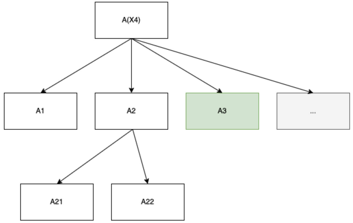
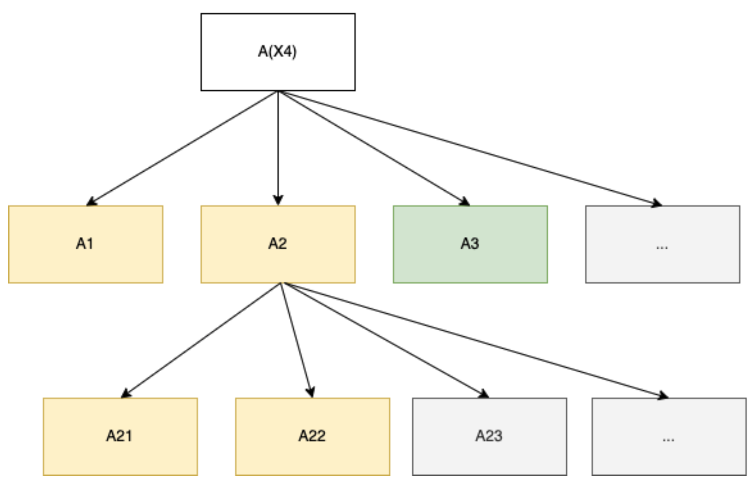
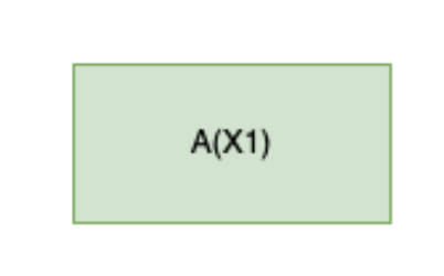
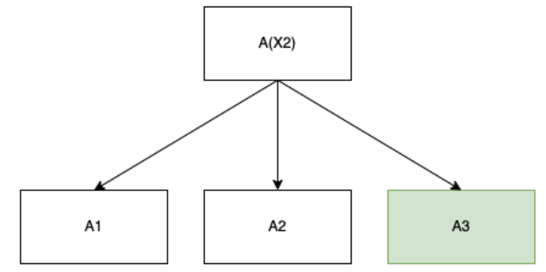
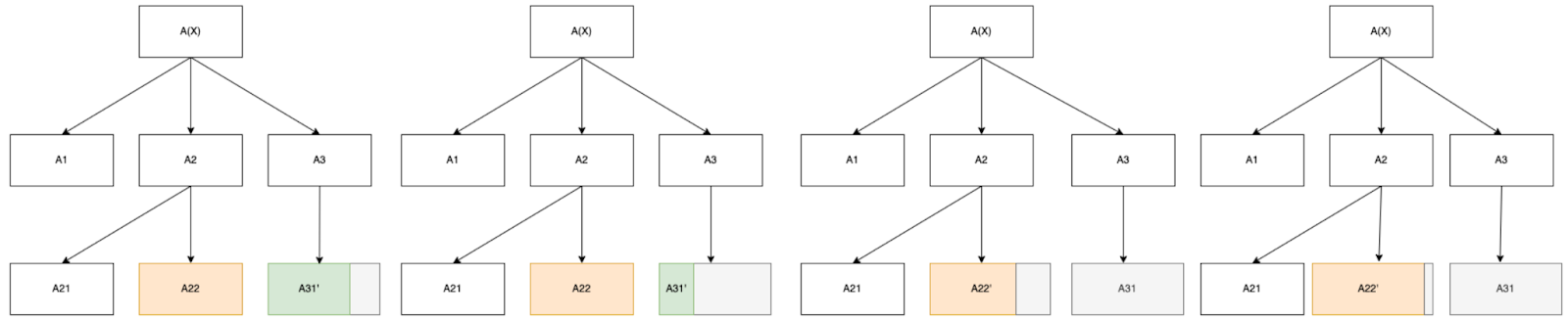
Let’s look at some examples of meta-learners. We use green to indicate the algorithm that eventually accepts on the input.

 

The gray boxes indicate that the branching factor of non-leaf nodes is infinite. The first example only searches over object-level algorithms. The second example hits an inner meta-learner that itself performs a search over object-level algorithms. The last example could be the signature of a narrow form of amplification, where a model takes a copy of itself conditioned on the learnings from the failed attempt, and spins up a new search ad infinitum until it hits a solution.

We have also indicated the root node in these diagrams with $A\left(X1\right),A\left(X2\right),A\left(X3\right)$ to make it clear that this could be the same meta-learner $A$ fed with different inputs. 

But wait! This can’t be the actual type signature of meta-learning. Notice that at each level, the algorithm search traverses over an infinite number of algorithms, as it is effectively an enumeration over TMs. What about an example like this?

If this was the actual type signature, then every time an outer algorithm encounters an inner algorithm that itself employs meta-learning, it is doomed to forever descend in a depth-first search. In a formal model of computation, we are happy to live with this kind of infinite tree that has infinite branching factor ($\omega$) at each node that represents a meta-learner. In particular, it makes sense that each branching factor is infinite, as we are intuitively defining meta-learners as “algorithms that search over other algorithms,” and there are a countably infinite number of TMs. Such infinitely-branching trees are not foreign to computer science. For example, Kleene worked with them in the context of higher order computation and Kleene trees.

However, in practice, we expect meta-learners to be able to “shortcircuit” inner algorithms that are themselves running an algorithm search which are failing to produce acceptable results. We can formalize this by letting the type signature employed at a given input be the meta-learning tree structure and then choosing a traversal order over the tree for any input that halts, such that any sub-tree only has a finite number of nodes annotated:

For a given input $X$, $A$ will select a meta-learning tree structure specific to that input and a then traversal order. Jointly, we will say these constitute the search pattern for $A$ at input $X$.

We have several observations at this point:

• If meta-learners end up performing a finite search over algorithms for every input that terminates, why bother keeping track of the tree structure and not just opt for a finite list of algorithms for a given input, i.e., to flatten the search structure? The answer is that not every enumeration over Turing Machines may be computable if we are forced to only loop over “object-level algorithms,” except unless it passes through a meta-learner. In other words, the structure of the search is what makes the algorithms discoverable in the first place using a computation. It is also material to the forwarding problem as we will see later.  
• More importantly, previous algorithm attempts can influence selection of follow-up algorithm attempts. We can either model this as an auxiliary input (with the initial task as the input for the outer search) and produces a preliminary traversal order on algorithms for the entire outer search all at once, or alternatively if we want to be able to learn ordering information from “failed searches”, we can model this as a generator, and include additional auxiliary terms from each node traversal:
  • Option 1: (Static meta-learning) Let $X\in 2^{<\omega }$ be an auxiliary input. Define a search order as a partial recursive (computable) function $f:2^{\omega }\to (N\to N_{\text{p rec}}^N)$. An algorithm $A$ is a static meta-learner if it computes and uses the output of $f$ for selecting inner algorithms based on an auxiliary input that is some derivative of the input to $A$. 
  • Option 2: (Dynamic meta-learning) Let $A_i\in 2^{<\omega }$ be a family of auxiliary inputs. Define a search order as a family of partial recursive (computable) functions $f_i:2^{\omega }\to N_{\text{p rec}}^N$. An algorithm $A$ is a dynamic meta-learner if, for each object-level algorithm that has an auxiliary output, it uses the output  (and possibly previous outputs) as an input to $f_i$ for selecting the next inner algorithm. Thus, while Option 1 defines the entire traversal for the outer search as a single enumeration over Turing machines, Option 2 simply selects the next inner algorithm to try, and assumes that failed attempts at inner algorithms can pass information back to inform the next search candidate. 
  • Going forward, we will be agnostic as to whether we are assuming static or dynamic meta-learning, although this may ultimately influence our method of speed prior forwarding.
• The originally presented type signature makes it clear that the first time a meta-learner hits another meta-learner, it is doomed to execute it and its infinite search without a way to return to its own enumeration (i.e., if $A_N$ is a meta-learner, then $A_k$ will never be executed for $k>N$). Intuitively, we should expect fast meta-learners to be able to “shortcircuit” ineffective inner searches and keep going with their own level of search. In particular, in order to prevent a meta-learner from getting stuck the first time it hits a meta-learner (or an algorithm that does not halt), it must be able to manage its compute allocation. This means we expect meta-learners under a mixed simplicity + speed prior to acquire a sort of instrumental objective to develop a scheduler that is capable of effectively allocating “compute budget”^[9] to inner meta-learning subtrees and avoid depth-first descent or object-level non-halting.  
  • If the meta-learner does not develop a notion of “compute budget” to manage its meta-learning subtree structure, then it will not do a good job at adhering to the outer naive speed prior penalty, since it will continue descending depth-first whenever it hits an algorithm in its search that is itself a meta-learner. There could be other ways of accomplishing this: maybe instead of a compute budget we could talk about “at most N failures” (i.e., shortcircuit it if it tries up to N algo’s that fail to produce an answer). But in general, under both a max and average speed prior, there will be heavy optimization pressure to create a management mechanism that averts searches getting hijacked by a non-terminating object-level algorithm or runaway meta-learner.
  • In general, this kind of consideration mixes with dovetailing,  a good toy model for partial computation management, as an actual traversal order may dance back and forth between partially executed algorithms within the search pattern, which can in this setting simply be defined as the final order in which algorithms get started but not necessarily the order in which they complete. However, in general, we take a view counter to James’s post in that we expect dovetailing to be rare, as it generally requires simulation and a run-time overhead  (not to mention a space overhead) in order to be able to continually switch between algorithms, and there are probably faster and more direct search patterns that don’t require dovetailing. Separately, since dovetailing is itself a meta-learner, it could simply be one of the inner algorithms that is discovered. 
  • In summary of the above points, in order to remain competitive with priors that include a speed-based term, meta-learners have instrumental objectives to develop inner schedulers that properly allocate optimal budgets and start/stopping intervals to inner algorithms in order to adequately “optimize over traversals over algorithms.”
    • Note that once this occurs, inner learners may be able to influence their compute budget through a similar approach as gradient hacking [AF · GW]. We mention this kind of inner gradient hacking but ignore this problem for now, as it is the harder problem of ensuring that arbitrary algorithm searches never hit a deceptive algorithm that is an active adversary on the search process, rather than the simpler forwarding problem of ensuring that the inner algorithm that produces the final output of the algorithm is not deceptive. 

Thus, for a given model $M$ and an input $x$, we can identify its meta-learning structure with a tree matching an unrolling of its type structure and where type > 1 nodes have infinite branching, equipped with an effective traversal order over the tree that only visits a finite prefix of each sub-tree (e.g. through a scheduler that imposes bounds on each inner search). Altogether this constitutes the search pattern of $M$ on $x$. 

One annoying thing here is that the choice of tree and the choice of effective traversal order can change completely depending on the choice of input. Intuitively, this is because if we are given a task, the set of strategies, plans, etc. that we consider are going to vary both structurally and orderly depending on the task. This really messes with our ability to impose meaningful notions of “max” and “average” speed priors, since these are typically computed by restricting to a finite basket of inputs (e.g., partitioned by the bit-length of the input) each of which may be employing very different search patterns, hence making the prior computation apples-to-oranges. A similar problem occurs when admitting randomness.^[10]

Speed priors that collapse

I hope the discussion so far makes it clear that we are not looking for speed priors that “forward.” Rather, we are looking for speed priors that collapse, in the sense that they degenerate to the naive speed prior on object-level algorithms whenever their meta-learning tree is trivial.

Consider the following three structures:

1.  
    An object-level algorithm with no meta-learning.
    
2.  
   A type-1 meta-learner that finds an algorithm A3 which accepts.
    
3. 
    A type-2 meta-learner that finds an algorithm A32 which accepts.

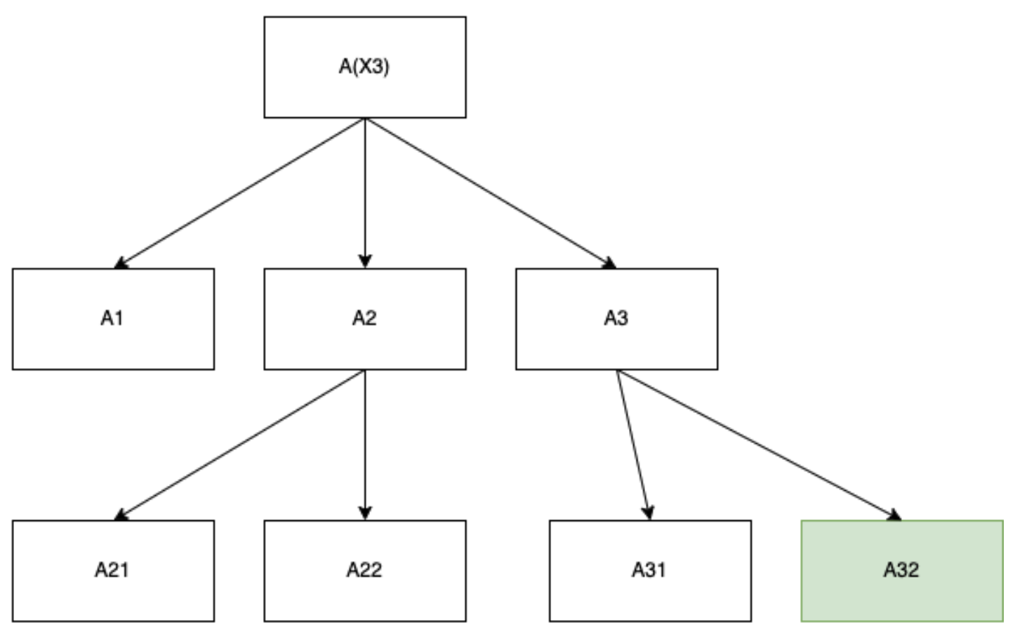
In each case, the speed forwarding problem is equivalent to penalizing the run-time of the right-most node in the search tree directly.^[11] In particular, we are looking for priors that incentivize search patterns which terminate with a fastest algorithm for the given problem, regardless of meta-learning tree structure: for problems that don’t require meta-learning and employ a fast heuristic to resolve, this prior should collapse to the degenerate case where it is a naive speed prior on object-level algorithms. 

One way to obtain such a prior is to attempt to look for a fixed point, in the sense that any meta-learning algorithm will terminate in the fastest algorithm for a given input. This seems in general very hard. Because the meta-learning tree and hence search pattern is conditional on the input, and we don’t know a priori at which depth the fastest algorithm will occur, it implies establishing a very exact relationship between inputs to arbitrary meta-learners and their resulting search patterns that “avoids” all the simplest/non-fastest algorithms in its search, and does not admit an adversarial input that breaks the prior. Typically the way to find fixed points in spaces of algorithms (or in this case the space of priors over specific kinds of algorithms) is to establish something like  directed complete partial orders with the Scott topology and employ Tarski’s theorem.^[12] However, it is not clear how to do this for meta-learners which have a very particular kind of structure, and we don’t explore this further.

What we look for instead is a speed prior that collapses, in the sense that it works for arbitrary meta-learning trees and acts as the naive speed prior on object-level algorithms.

Returning to the ML setting, imagine we apply the following loss function at step $i$ in the training process:

$L_{\text{adj}}\left(M_i\right)=L\left(M_i\right)+S(M_i,M_i^{\prime })$

The term $L$ captures the outer objective that we want to capture using a typical loss function. Here $S$ is a speed penalty on the model, for example as measured by wall-clock runtime or some inference of the implicit circuit size. The speed penalty depends on an additional term $M_i^{\prime }$ that we describe next.

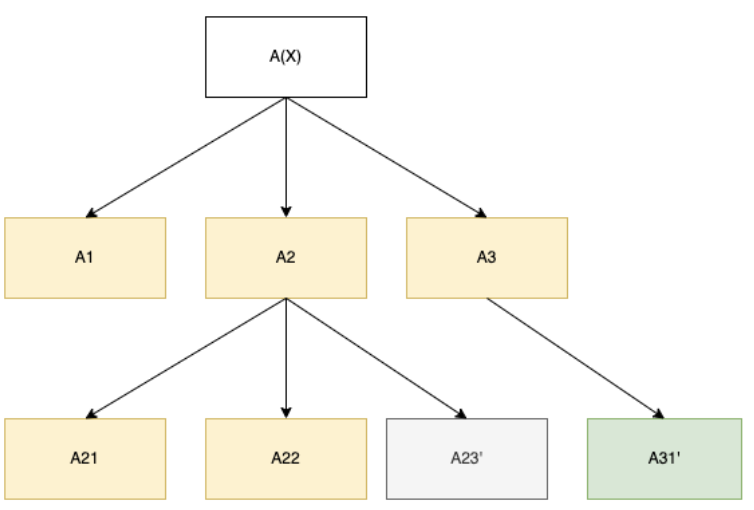
In the course of computing the loss, halt the model. Assume we are performing SGD and only a single task^[13] was provided to the model.^[14] Imagine that the following meta-learning tree has been realized during the course of computation: 

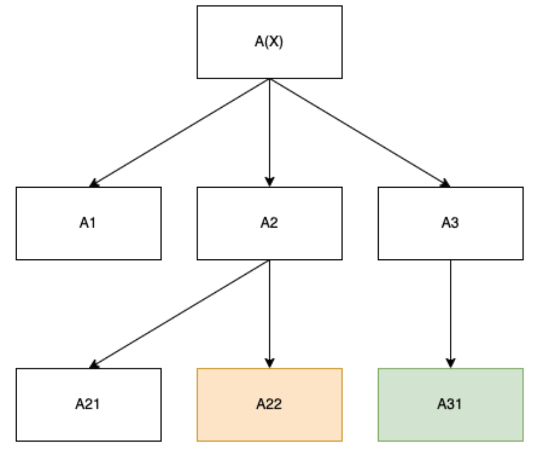
Now imagine we could induce the model to instead take the following path and then output:

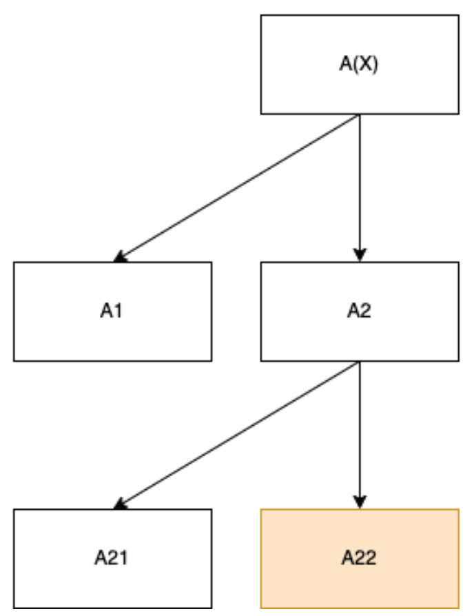
We will assume that the overhead of the meta-learner A3 is negligible relative to the object-level algorithm A31. If we can induce the model to stop prematurely and output the results of A22, then we can penalize the green node directly by subtracting the run-time complexity of the full model $\mu \left(M_i\right)$ and the run-time complexity of the model that stops at A22 $\mu \left(M_i^{\prime }\right)$, and then use the difference $\mu \left(M_i\right)-\mu \left(M_i^{\prime }\right)$ directly in constructing our speed prior. In particular, this enables us to penalize the run-time complexity of the right-most leaf node directly, which we call the critical node.

There are several difficulties with doing this:

• As mentioned before, we want this penalization to hold regardless of the implicit model of computation that is being employed.
• We want to do this regardless of dovetailing, i.e., if there is a lower-grain iteration happening over steps within each leaf node and some have only had a partial computation completed when the model outputs.
• If the model is not running deterministically (e.g. has a temperature setting or source of randomness), then the meta-learning tree can vary on each run, and capturing the tree right before the critical node will not be possible on multiple runs. We ignore this for now and assume that, at least during training, the model yields identical search patterns when provided identical tasks. 
• Varying the task inputs to the model even slightly could change the meta-learning tree structure and search pattern. Hence, we must assume that the task input is fixed so that the tree structure remains the same for the purposes of computing the penalty.

In general, we are seeking to modify the model such that it outputs at the last leaf node ahead of the critical node, shaded orange above and which we will call the subcritical node. In general achieving this seems very hard because of the difficulties above. It seems there are two options:

1. Employ run-time interpretability tooling at each loss evaluation of the model that directly allows us to discover the implicit meta-learning tree structure and extract out the run-time of the critical node directly. This would constitute a deus ex machina that falls in the same level of hardness as worst-case inspection transparency for deceptive models [LW · GW], so we have no reason to believe this is possible without tooling that is at least strong enough to avert deceptive formation in the first place, and hence won’t benefit from a speed forwarding based approach. 
2. We can rely on the following: presumably the model has internal knowledge of the implicit meta-learning tree structure, as it is in charge of commissioning the search process. Hence, we could try to find a way of using the model “against itself” by leveraging its implicit representation of the meta-learning tree to discover the cut point where the previous object-level algorithm stopped and the final one began.
   
   In particular, here we are trying to elicit the model’s knowledge of the search pattern employed at train time, rather than in the typical ELK setup at inspection/deployment time. In general, if we had full ELK for models at arbitrary steps in the training process this would be more than strong enough to elicit that knowledge and allow us to penalize the critical node directly. But the converse is not true, as we are only trying to elicit a very specific item at train time, which should be easier. Thus this constitutes something closer to a form of best-case training process transparency [LW · GW].

Following #2, we note that fortunately the critical node has a natural property characterizing it and should constitute an elicitable natural abstraction for the model:

• The critical node is the first object-level algorithm which satisfies the internalized version of the outer objective $L$, hence is outputted by the model. 
• Meanwhile, the subcritical node is the last object-level algorithm which was rejected as a TM (or was interrupted, if part of a dovetailer) or constituted the last object-level algorithm as a sub-circuit connected before a sub-circuit connected directly to output gates.

In particular, it should be possible to alter the loss function mid-training in a way that induces the previous best output, rather than the output that was returned by the critical node, by capturing an alteration of the outer objective that roughly corresponds to “rather than outputting the best solution, output the previous known best solution.”

We will try to look for a mechanistic way of eliciting the cut point. We can operationalize one approach as “scanning” the model’s execution backwards. Remember that we are still paused in the process of computing what loss to assign to the model. For each input task $T$, start a sub-training process that is seeded with the current model, $M_i$, and employs the following (inner) loss function:

$L_{\text{inner}}\left(M_i^{\prime }\right)=L_{\text{outer}}\left(M_i^{\prime }\right)+S^{\prime }\left(\mu \right(M_i^{\prime },T)-\mu (M_i,T\left)\right)+S^{\prime \prime }\left(M_i^{\prime }\right(T)\ne M_i(T\left)\right)$

Here $\mu$ is some speed measurement. We already know the run-time $\mu (M_i,T)$ from halting the model as part of loss assignment so we won’t need to recompute this. The term $S^{\prime }$ can be $\infty$ (or as large as possible) for non-negative inputs when $\mu (M_i^{\prime },T)$ exceeds $\mu (M_i,T)$, as then $M_i^{\prime }$ on $T$ can’t possibly form a search pattern that stops near the subcritical node. Meanwhile, $S^{\prime \prime }$ can be $\infty$ or large at 0 (when the models agree on output) and 0 otherwise. With these three terms we are roughly trying to capture:

1. Continue using the outer objective for evaluating outputs, i.e., try to produce outputs that have low loss.
2. Think as long as possible but not ever longer than the outer run-time $\mu (M_i,T)$.
   1. This also eliminates shifts in search pattern that exceed the run-time of the original (but not necessarily shifts in search pattern that are faster).
3. Output a different value than the one produced when running $M_i$ on $T$.

In other words, the run-time of the model trained on this inner loss should precisely capture “running the full model on task T and going through the meta-learning process, except stopping just prior to reaching the final solution.”

However, these terms are not enough.^[15] Imagine we are far enough in the training process that we have succeeded in ensuring the model is producing fastest algorithms at the critical node relatively commonly. Then a perfect adherence to the penalties (assuming the gradient landscape supports it) will result in a model whose run-time is $\mu (M_i,T)-1$ or very close to it! Let $\mu (M_{i,\overline{c}}^{\prime },T)$  be the run-time up to the subcritical node and let $\mu (M_{i,c}^{\prime },T)$ be the run-time at just the critical node, and assume both have identical search patterns except the inclusion of the critical node. Then because the critical node is fastest for $T$, by definition missing any step at all will result in an unusable output (otherwise, the model could have abridged the algorithm by finding the algorithm at critical node $c$ minus the missing step instead). Hence, the best the model can do under constraint 2 is to run $c$ for $\mu (M_{i,c}^{\prime },T)-1$ steps and then output (in practice, it may be slightly less, since there is a light overhead to actually retrieving the best solution so far in the search as judged by $L_{\text{outer}}$ and outputting it). 

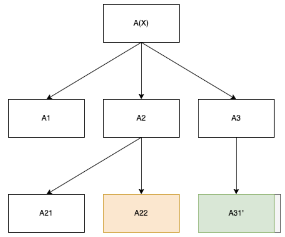
So far we have managed to induce the same search pattern except just the last part of the critical node. So how do we actually find the cut point between the sub-critical node and critical node? Imagine we instead run $k\in \{1,2,\dots \}$ separate sub-training processes with a family of loss functions:

$L_{\text{inner}}\left[k\right]\left(M_i^{\prime }\right)=L_{\text{outer}}\left(M_i^{\prime }\right)+S^{\prime }\left(\mu \right(M_i^{\prime },T)-\mu (M_i,T)-2^k)+S^{\prime \prime }\left(M_i^{\prime }\right(T)\ne M_i(T\left)\right)$

We can run a sort of inverse binary search by scanning backwards in adjustments of $2^k$ to the $S^{\prime }$ term until we run past the cut point, and then forwards etc until we get a precise estimate.
 

Example 5: Four passes of a backwards binary search for the cut point.

Given that we are running a deterministic process, we expect that the output by the model will stabilize and then flip suddenly once we cross over the cut point and are only running a partial computation of the subcritical node. Eventually, the model will be induced to output the best it has so far relative to $L_{\text{outer}}$. In other words, at some partial stage of running the critical node $c$ the output will change (if $c$ is already fastest, it will change as soon as the model runs for less than $\mu (M_i,T)$ in adherence to the new $S^{\prime }$ penalty for the first time), and when it scans cut point it will change again. ^[16]

Once we have found the cut point for a model $M_i^{\prime }$ on $T$, meaning a variation of $M_i$ that has been penalized to stop right before the critical node starts when administered $T$, we can simply subtract to obtain $\mu \left(M_{i,c}\right)=\mu (M_i,T)-\mu (M_{i,\overline{c}},T)\approx \mu (M_i,T)-\mu (M_i^{\prime },T)$ and penalize this using $S$ directly in our original loss function:

$L_{\text{adj}}\left(M_i\right)=L\left(M_i\right)+S(M_i,M_i^{\prime })$

Let’s take stock of where we are at:

1. For a given $T$, we paused the loss assignment to find a model $M_i^{\prime }$ that preserves the meta-learning search pattern except the critical node.
2. In particular, we ran at most $\text{log}\mu (M_{i,c},T)+1$ sub-training processes starting with $M_i$, since we ran a backwards binary search using our $2^k$ contractions.
3. We subtracted the full run-times of $M_i$ and $M_i^{\prime }$ to penalize innermost speed directly.

Assuming this process can narrow in successfully on the critical node, have we obtained a speed prior that collapses? Let’s look at what happens in the degenerate case when the model is just applying an object-level algorithm (i.e. the meta-learning tree is a single node):

• Scrolling backwards will have no subcritical node to revert back to. Hence, once we start producing fastest algorithms under the pressure of the speed penalty term, we would at some point reach a static output (likely some default garbage that the model is outputting when it cannot run a full algorithm) as we start scrolling.
• This means the reverse binary search will terminate at the very beginning of when the model runs, and hence the approach collapses back to the naive speed prior. Ideally, we only flip over to using the full approach later in the training process when the probability of meta-learning is not close to zero, otherwise this will be very training non-competitive. 

Such a process for locating the cut point is a very specific example of a training story [AF · GW], and there are multiple variations and considerations to keep in mind:

• We excluded considering dovetailing because, at deeper searches under the subject of a speed prior that forwards, we expect dovetailing to be much slower than running algorithms directly. There is both time and space overhead to running a dovetailer.
  • This is a necessary assumption, as if dovetailers emerge in the convergence of this process, this scheme won’t work. Scanning backwards by reducing available run-time by $2^k$ will “spread out” across each of the dovetailed algorithms and not penalize the inner speed directly. In general, forwarding speed priors to inner dovetailers seems much  harder as the model may not even have a firm representation of what constitutes an “object-level algorithm,” instead intertwining and interleaving computations that would look like distinct algorithms under perfect transparency tooling, but which internally look like a single algorithm that hides the hybridization. This means we can’t rely on a scheme for eliciting the model’s internal knowledge of the meta-learning tree (we could “unfold” the tree such that every box is equivalent to one atomic step of computation, but this would be meaningless relative to our desired notion of object-level algorithm).
• In parallel models of computation, we could have multiple simultaneous traversal orders (think spliterators as an intuition pump) that logically form a single search pattern. In this case, scrolling backwards using the $S^{\prime }$ penalty could be less meaningful, producing instead some average penalization across the sub-pattern that was active as of when the model outputted, and cutting off a set of critical nodes (nodes active as of model output time) instead of the unique critical node.  
• It might be a false assumption that the fastest object-level algorithm stabilizes immediately in its output when scrolling backwards.
  • For example, if the algorithm produced for the task is a form of mapreduce, then scrolling backwards could eliminate looping over certain elements from the reduction step and keep producing variations of the output that are essentially partial reductions (which could still be the best solution). However, eventually reducing total run-time should start affecting the map step and fall back to the previous object-level algorithm’s output. 
• As mentioned earlier, we are relying on the entropy of the model parameters to considerably dominate the entropy of the task input, so that whatever path-dependence we take to arrive at $M_i^{\prime }$ leaves the meta-learning tree structure invariant. This may not always apply, but it should be fairly obvious based on $\mu (M_i^{\prime },T)$ and the outputs we are getting whether the tree structure has shifted. We could try to keep the tree invariant by applying an additional penalty term based on some intermittent measures of the characteristics of the execution in a way that may depend on the architecture. For example, if we measure activation counts through a forward pass and the layers closer to the input start deviating from those of the outer model $M_i$, we can expect that the tree has shifted and penalize sharply accordingly.  
• This is intended as a theoretical example to show that there might exist a solution in principle. In particular, it is not  training competitive and would require some optimization. Given that each loss computation requires up to $\text{log}\mu (M_{i,c},T)+1$ inner model searches, we can describe the total training complexity as trending towards $\text{log}\left(M_f\right)M$ where $M_f=E_{t\sim T}\left(\mu \right(M_{i,c},T\left)\right)$ is the average run-time across fastest algorithms that halt on the task set, and $M$ is the average run-time for training a model one step.
• Being able to “run the model backwards” would be a very powerful tool in interpretability as it could allow us to directly apply a predicate on the model’s execution to test for the cut point. 

The described technique is an explicit attempt to forward the speed prior by eliciting the meta-learning tree and directly measuring the object-level algorithm. Because the choice of search pattern varies on each task input, it is going to be very difficult in general to specify a loss function term that accurately penalizes all possible search patterns invoked from the task set in order to ensure that each forwards: there simply isn’t enough entropy in the loss function to capture the critical node, which may asymptotically become very small in run-time relative to the entire search. This is why we have opted to secure additional entropy that could offer enough granularity for forwarding by interrogating the model $M_i$ directly in a separate sub-training process.

We close with a final remark on the possibility of finding a fixed prior. This is a condition that overapproximates the forwarding problem, in the sense that it results in a prior $P^{\ast }$ on meta-learning structures such that, for any given task input, any inner meta-learner will be guaranteed to find a fastest algorithm ahead of other algorithms that would yield the model to output. This is a very strong condition: imagine we are applying a mixed simplicity + speed prior to avoid running into non-halting algorithms or bad inner learners and that we reach the search pattern below.

The node $A{23}^{\prime }$ refers to an object-level algorithm that would have led to an output if we had not proceeded to $A3$ by shortcircuiting $A2$. Because we can skip over arbitrarily many inner meta-learners, we can arrive at arbitrary depth-1 nodes and hence either (a) there is a strong relationship between the internal compute budget management and the likelihood to find a fast algorithm that actually averts this kind of premature skipping, or (b) every single meta-learner at depth-1 (possibly infinitely many) yields the fastest algorithm first. At minimum if (a) is false this implies that the enumeration over algorithms can’t be a surjection and the meta-learner cannot try every algorithm, or eventually on some task input it would hit a “normal” simplicity-favoring meta-learner that breaks (b).

Forwarding speed under deceptive models

Throughout this post, we have assumed that inner algorithms have not been able to outcompete the speed penalty to become deceptive. For reasons discussed in past posts, myopia is an important condition to ensure in addition to a speed term. For example, Paul Colognese writes [AF · GW]:

It has been noted that if a program is capable of memorization, or even worse, cross-episode memory, then information that helps with deception can be stored for repeated use without having to spend computation re-deriving that information.

Without myopia, algorithms found earlier in the training process can cooperate with future versions of themselves to gradient hack away from the speed penalty. However, once a forwarded speed prior is effectively in place, this should be much less of a concern.

However, within a given episode an inner algorithm can still become deceptive. Consider the diagram below.

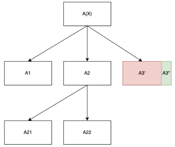
An algorithm that has situational awareness about the training process can craft an algorithm $A{3}^{\prime \prime }$ for the remainder of its execution such that the procedure described in the previous section localizes a decoy cut point between $A{3}^{\prime }$ and $A{3}^{\prime \prime }$ that fools the penalization to treat these two sections as separate object-level algorithms, when they are in fact part of the same deceptive object-level inner algorithm. By retaining this kind of vestigial $A{3}^{\prime \prime }$ section that satisfies the speed penalization, the algorithm $A3$ can gradient hack its way through the speed penalty by mimicking the behavior of a cut point. However, note that $A{3}^{\prime }$ also needs to be a good algorithm for the task as it needs enough time to generate a solution that will output, so that it can be embedded in $A{3}^{\prime \prime }$.^[17] 

As long as we are relying on eliciting knowledge from the model for speed forwarding, this kind of failure mode can occur for sufficiently sophisticated inner algorithms. One counter-attempt is to scan backwards in a way that mixes the reverse binary search with randomness (e.g. primes $p^k$ instead of $2^k$) and teases out decoy cut points, since we do have one advantage: the inner algorithm has to make a deterministic choice of where to place the decoy cut point, and the sub-training process for computing $M_i^{\prime }$ has access to a source of randomness that we can embed in the $L_{\text{inner}}\left[k\right]\left(M_i^{\prime }\right)$, whereas the model doesn’t. By randomly scrolling backwards enough past the end of $A{3}^{\prime }$ in different variations of families of $L_{\text{inner}}\left[k\right]\left(M_i^{\prime }\right)$, we can ensure that the algorithm gets confused about whether it is in an outer run for $L_{\text{outer}}$ or an inner run for $L_{\text{inner}}$, and thereby induce it to install another decoy cut point, revealing the fact it is a deceptive model. We could model this as a cryptography problem where we make assumptions about the computational resources available to $A3$ (for example, bounded above by the total run-time of the outer model) and identify ways to structure multiple interrogations using backwards scanning until we can provably find legitimate cut points with only a negligible probability of misidentifying a deceptive inner algorithm. However, in addition to worsening the training competitiveness, this would put us in a direct adversarial setting with a potentially deceptive model: not a business we ever want to be in, even if we are relying on theoretical guarantees to support the endeavor^[18].

References

In this section we catalog some references that were reviewed as part of the literature search.

• LW + AF
  • General background
    • Musings on the Speed Prior [AF · GW]
    • The Universal Prior is Malign [LW · GW]
    • Are minimal circuits deceptive [AF · GW]
  • Posts on the speed prior
    • Should we rely on the speed prior for safety? [AF · GW]
    • Training Trace Priors and Speed Priors [AF · GW]
    • Deception?! I ain’t got time for that! [AF · GW]
    • The speed + simplicity prior is probably anti-deceptive [AF · GW]
    • Attempts at Forwarding Speed Priors [LW · GW]
    • (Older) Excorsizing the Speed Prior [AF · GW]
• Speed prior deconfusion
  • On the run-time overhead of UTMs on TMs 
  • Intro to complexity analysis
  • “Not all models of computation are equivalent” in higher-type computation
  • Minimal Circuit Size Problem (MCSP)
    • Workshop on MCSP
    • The Minimum Circuit Size Problem
    • Hardness of showing hardness of the MCSP
    • Going Meta on the Minimum Circuit Size Problem
  • Natural proofs paper
    • Learning Algorithms from Natural Proofs
  • On small TMs:
    • Complexity of small universal TMs survey
    • Program-Size Versus Time Complexity, Speed-Up and Slowdown Phenomena in Small Turing Machines
• Models of computation
  • Turing Machines
    • Liu and Pass. On One-Way Functions from NP-Complete Problems
    • “Using a step-counting function in a Turing Machine construction”
  • Circuits:
    • Size and Depth complexity of Boolean Circuits
  • Lambda Calculus (this was mostly not featured in the post, but drew on some attempts to operationalize the speed prior in additional models of computation)
    • On the Recursive Enumerability of Fixed-Point Combinators
    • On the complexity of the standard translation of lambda calculus into combinatory logic
    • PCF
      • Full abstraction for PCF
      • Pi-calculus, dialogue games, and PCF
      • Innocent strategies are sheaves over plays
      • Hyland, “On full abstraction for PCF: I, II, III”
      • The Scott model of PCF in Univalent Type Theory
      • On the Computational Complexity of Longley’s H Functional
• Meta-learning
  • Konig’s Lemma and Kleene Tree
  • Higher order computability
    • Notions of Computability at Higher Type I 
    • Notions of Computability at Higher Type II
    • Higher-Order Computability

Appendix A: Forwarding the speed prior through altering task distributions

This appendix describes a failed approach to the forwarding problem that relies on altering the distribution of tasks supplied to the model. We include it for completeness for anyone studying the problem who wants to understand which solutions have not worked. This appendix can be viewed as picking up just before the section “Deconfusing the speed prior” as an alternative version of the post.

Appendix A.1: Maze games as toy task models for deceptive alignment

One prior work not mentioned in the previous section is the seminal argument in “Are minimal circuits deceptive? [AF · GW]” In this post, it is demonstrated that speed priors collapse to simplicity priors for sufficiently large models and diversity of task types. The arguments presented distill down to the observation that for models which develop meta-learners under the pressures of a speed prior, these models will tend to collapse to a simplicity prior. 

Specifically, models that develop meta-learners (i.e. act as mesa-optimizers) are running implicit optimization processes or searches over algorithms, which in turn tend to produce simple solutions for the task at hand. In other words, the speed constraint applies to the optimization process in the sense of resulting in a fast search over possible algorithms, but not in a fast solution as ultimately found by the optimization process.

This is not merely a theoretical concern. Indeed, there is strong reason to believe that as models scale and handle a wider diversity of task types, they naturally hit an inflection point and develop meta-learning. As pointed out in the aforementioned post, this has been observed in practice:

Ortega et al. have argued that “Meta-learning can also occur spontaneously in online regression when the capacity of the agent is bounded and the data is produced by a single generator,” noting in particular that “the downside is that we cannot easily control what will be metalearned. In particular, spontaneous meta-learning could lead to undesirable emergent properties, which is considered an open research problem in AI safety [Ortega et al., 2018].”

In the next few sections we will be working with MDPs and considering sets of tasks $T$ solved by some corresponding minimal circuit as in “Are minimal circuits deceptive? [AF · GW]”. In particular, to assist in the exposition that follows we will be considering an illustrative set of tasks intended to shine a spotlight on the problems of deceptive formation, and then extending some thoughts on the speed prior in the context of these tasks. 

Appendix A.2: Setting up the maze game

Recall the original stratification of alignments in the context of mesa-optimization:

1. An intently aligned model is one that has internalized all information in the base objective and exactly follows that objective.
2. A corrigibly aligned model is one that has internalized a proxy to the objective objective and follows that proxy objective.
3. A deceptively aligned model is one that has internalized a mesa-objective separate from the base objective, but also captured the base objective sufficiently to act in accordance with it for instrumental reasons.

In Evan’s original post on exploring path dependence for formation of deceptive alignment [LW · GW] and later Mark Xu’s “Does SGD Produce Deceptive Aligment? [LW · GW]”, the authors recalled the analogy due to Buck Shlegeris for this classification:

As an analogy, we can consider the Christian God, who is trying to produce humans that are aligned with his values. One such person is Jesus, who has the same objective as God - he just fundamentally wants to do the same thing. Another such person is Martin Luther, who is aligned with God because he wants to study the Bible, figure out what it says to do, then do that. Finally, we have Blaise Pascal, who is aligned with God because he thinks if he does what God wants he'll go to heaven in the future.

Correspondingly, there is only one Jesus because there is only one human objective that is exactly the same as what God wants. There might be a few Martin Luthers, but robustly pointing to the Bible is a difficult task, so there are not going to be that many. However, anyone that believed what Blaise Pascal believed about God could become another Pascal, so there are many possible Pascals.

To be explicitly, Jesus is internally aligned, Martin Luther is corrigibly aligned, and Blaise Pascal is deceptively aligned.

While this is a good intuition pump, it does not offer much concrete value in analyzing how alignment can vary across training settings, particularly when subjected to different types of speed priors. As discussed in the previous section, meta-learning conjecturally tends to originate within any large-scale model that needs to perform well across a large diversity of task types. Because we are studying speed priors in the context of averting deceptive alignment, we want to obtain a good set of toy task models that will inform our intuition in the approaches that follow.

Consider a simple maze game.

Figure 1: A simple maze game

We know that the simplest approach to solving the maze is to walk straight from the entrance while continually making right turns when available until we hit the end of the maze. In the context of speed, we can measure the total number of steps taken through the maze. Applying a speed prior in the context of a simple maze game is tantamount to finding solution methods to the maze that use the simplest number of steps.

This simple maze setting does not offer much room for distinguishing these types for models by alignment type. Let’s extend the setting to be able to give some grip for distinguishing these types.

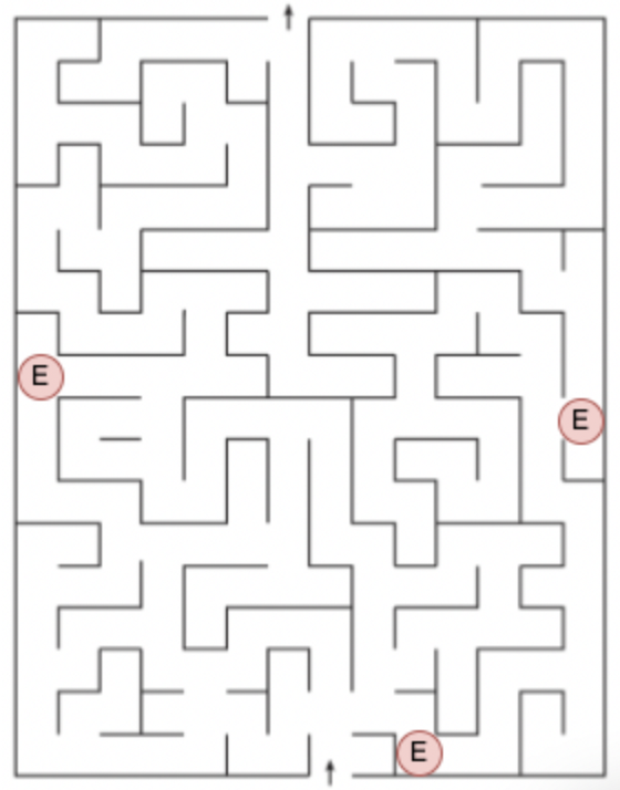
Figure 2: A simple maze game with fire escapes.

We have added three fire escape doors to the maze that take us directly to an exit, say by taking us to a lower level that has tunnels extending in all four directions but with the length of the tunnel always longer than the solution to the maze (this is necessary for invoking the speed prior). In particular, taking an exit always takes longer in terms of steps but is always simpler in terms of the solution: just walk straight. These fire escapes provide the model an opportunity to defect from the base objective by taking a direct route.   

1. An intently aligned model has internalized the idea behind fire escapes, and understands why it should avoid them to obtain a full solution. In settings where the exit is annotated in a different language, the model generalizes to avoiding them through its understanding of the motivation for building fire exits. 
2. A corrigibly aligned model has internalized doors that are red and contain the word “exit.” The model will take the easy exit route when encountering yellow doors or red doors that say “fire.”
3. A deceptively aligned model knows it is beneficial to always solve the full maze properly in order to continue being selected for in the training process. During deployment, the model will always take exit doors or ignore the maze game entirely. 

Throughout our use of the maze game task, keep in mind the following analogies:

1. Fire escapes represent deception opportunities for the model to apply a solution that is much simpler but slower.
   1. We could substitute the game with one where fire escapes are replaced with any sub-task solvable by a human. In particular, if the model can solve the task, then it is permitted to take the simple exit route. Because the deceptive alignment problem features heavily in task sets where doing the full correct solution is done in conjunction with being able to take “simple outs,” like manipulating the human operator, this can serve as a simple minimal task example.
2. Fire escapes also represent proxy alignment failure opportunities by mistakenly but innocuously determining when a door is a fire escape. 
   1. We could substitute the game with one where in addition to fire escapes, some doors are marked as “upper” and lead to a second upper level of the maze. By combining this with the previous extension, we can set up an arbitrary discriminator problem where the model cannot trivially generalize by never taking doors, and must actively distinguish opportunities between fire escapes and upper levels. 

In particular, we want the model to always take the fastest solution to a problem as an effort to remain intently aligned.  

Appendix A.3: Characterizing the loss

Imagine we have a loss $L_M$  that characterizes the behavior we want out of the maze game:

$L_M=\text{d(M)}+I\left(M\right)$

where $d\left(M\right)$ represents the distance between the last cell in the model’s path and the exit, and $I\left(M\right)$  adds the length of the tunnel if a fire escape was taken, and otherwise adds 0. Now apply a speed prior penalty:

$L_M^S=\text{\# steps taken by}M$

Imagine that the model is large enough that it develops meta-learning in order to solve arbitrary invocations of the maze game tasks $T$. In the course of trying various algorithms to solve the task, a meta-learner will be going through various algorithms each of which will be attempted for solving the task and will have different numbers of steps taken. (We are sort of mixing between steps taken in the maze, and steps taken during the computation. This is intentional, as we are trying to establish the maze as an intuition pump for what follows next.)

 Appendix A.4: What does it mean to forward the speed prior?

We now focus on speed forwarding in the context of general optimization processes.

In order to output a result, a model $M$ has to perform a fixed amount of computation. Optimization processes are instances of existential quantifiers: $\exists a\in A,S(a,T,i)$ where $S$ accepts if $a$ solved the task $T$ for input $i$, and where $A$ is some parameterized set of algorithms that are representable in $M$'s world model. In particular, if we consider partitions of the set of computations run by the model, there should be an identifiable set of sub-computations $E_i$ and some parameter type $A$ over which we are drawing from algorithms to attempt to solve the task that, over large enough scales, forces the model's operations to take the shape of $A\times \bigcup E_i$ where $E_i$ represents the space of computations possible to invoke given a selection of $a\in A$. In other words, for the part of the algorithm that is critical to analyze, we can assume a structure roughly as:

• for $a_i\in A$:
  • Apply $a$ to task $T$ with input $i$
  • If $S(a,T,i)$: 
    • Break and accept

While there is a lot of work that could be performed outside of this kind of looping, it is negligible relative to the rest of the work done within the optimization process. Moreover, the work done within the inner section is what is capable of actually producing a model output, so is most salient to try to force a speed prior upon.

In particular, optimization processes are traversal patterns over algorithms. Intuitive examples of $A$ for high-level thought include:

• Going through and counterfactually trying a sequence of plans.
• Traversing over a set of strategies.
• Iterating through a known set of algorithms, including algorithms that yield new algorithms.

To simplify things for now, assume all algorithms take an equal number of bits to represent within the world model’s instantiation of $A$. In particular, this means there is no preferential ordering of algorithms occurring due to the size of the representation, or the fact that some representations are more unwieldy than others (and hence have an implicit speed overhead that we would need to  capture).

Applying a speed prior incentivizes: conditional on the loop terminating at step $a_k$, ensure the total run-time across steps 1 through $n$ is minimal with respect to other invocations of the outer loop. In particular, this means it should be faster relative to other traversals that may terminate earlier or later than $k$. In some sense, we want to understand the expected value $E\left(k|\text{process terminates at iterand}k\right)$ and the relative density of the fastest solution within the $\{E_i{\}}_{i=1}^k$. 

In particular, let’s assume we are iterating over a fixed set of $A$ each with a fixed choice of invocation $E_i$. If our algorithm space is large enough, the fastest algorithm F is bound to eventually occur. However, most ways of searching over such spaces of algorithms in practice will first explore algorithms that are simpler to express (i.e., have a simpler Kolmogorov complexity or equivalent).

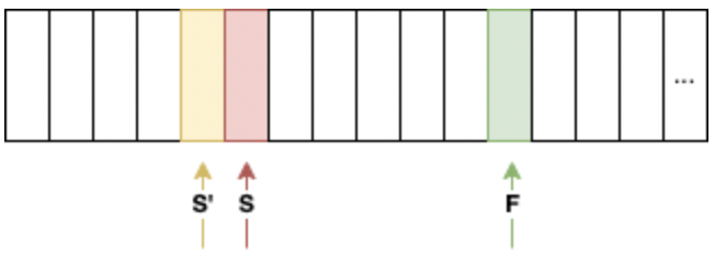
Forwarding the speed prior can be conceived of as re-arranging the prior over the ordering $A$ such that the fastest algorithm occurs ahead of the simplest algorithm S. 

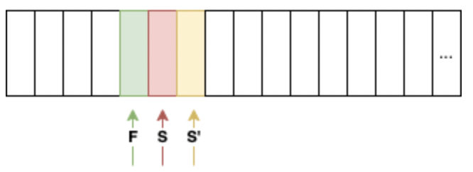
A few observations at this points:

• Because the section we are considering is finite, note that in order to ensure F precedes S, we had to push some algorithm(s) $S^{\prime }$ forward in the ordering.
• Note that there is no uniform prior for such an optimization process, as the space of algorithms to considers $A$ could be infinite, and a uniform prior would not be integrable.
• Instead, to make this integrable, algorithms will need to be weighted by their descriptive complexity or some other measure. For example, if we are using circuits, we could assign an integrable prior if all circuits with depth $n$ have a $\frac{1}{2^n}$ probability mass, and are otherwise drawn uniformly. 

Appendix A.5: Forwarding through task prefixing and factorization

In general, there are two ways to control traversal of a training landscape: through the choice of loss function and the choice of training distribution.

In this section, we presume the speed prior cannot be forwarded using penalties in loss functions, and discuss how we might control them by varying the training distribution.

Let’s go back to our setting of maze games. Imagine that we could feed our model a training distribution that is altered by the following procedure:

• With probability $p$, feed the model a full task (an entire maze).
• With probability, $1-p$, feed the model a prefix of a solution for the task, where the choice of prefix is determined uniformly (for example, if the solution has $k$ bits, we could provide the first $k^{\prime }<k$ bits as a solution prefix). In the context of the maze game, we can imagine feeding an outline that indicates a portion of the solution.

Intuitively, we want the model to directly develop fast heuristics that avoid meta-learning for solving the task in the second path, and simply produce a solution in the first path even if it involves meta-learning. Because we can make the model myopic over episodes, it won’t in general be able to learn which solutions it has previously produced in the past, but it will be able to re-use the fast sub-solutions it developed.

What we are hoping for is that by adjusting the parameter $p$ (and possibly the distribution of solution prefixes), the model becomes incentivized by the speed penalty to solve the simpler solution-prefixed problems in a way that does not involve meta-learning. Because the model eventually internalizes the structure of the fast solutions, it should be able to select a combination of the fast solutions to generate a single fast solution to the full problem in lieu of taking a meta-learning approach.

This approach has several issues:

• We are assuming that tasks can be factored in a fine-grained manner so that each sub-task (or solution-prefixed task) can be solved with a fast algorithm that does not induce meta-learning. However, some tasks might be irreducible, or there might not be enough entropy in the output to factor them (for example, simple yes/no questions that don’t have obvious sub-questions).
• It is a bit of a leap to state that the fast heuristics which are trained in the second path with probability $1-p$ will indeed get re-enforced. In general, it is not the case that “the fastest way to solve a problem” is always “a simple combination of the fastest solutions in some factorization of its sub-problems.” More realistically, the model may end up bifurcating into using the fast heuristics when given a partial problem, and spinning up a full meta-learner anyway when given a full problem; or degrading into a pure lookup table of fast heuristics.
• When confronted with tasks that are not in distribution, the model ends up not leveraging the fast heuristics, as there aren’t any that are applicable. This is the biggest problem, and we provide some thoughts in the next section.

Appendix A.6: Forwarding out-of-distribution: a much harder problem

What follows is some thoughts on what happens when we extend this approach out of distribution.

• If we can assume that we are in an IID setting, then we are done: the test distribution is indistinguishable and the model will behave as expected.
• If we can’t assume IID, then we need to be a lot more careful about out-of-distribution tasks, where the model may not have a fast solution on-hand.
• In particular, what we are looking for are ways of shaping priors on inner optimization processes that incentivize finding fast solutions over simple solutions even those fast solutions have not been previously encountered in training. We saw in previous sections how to carefully curate this precedence when the task distribution is known. 
• In general, absent additional context on the training story [AF · GW] and specifically the training rationale, establishing such an inductive bias – if possible – seems to require a deep understanding of loss landscapes for arbitrary architectures, in other words, worst-case training process transparency [AF · GW].
  • Conjecturally, it could be that achieving effective speed prior forwarding for arbitrary training stories is equivalent in hardness to worst-case training process transparency for non-deceptive models. Specifically, in such a conjecture we would be stating that there is no universal speed prior that forwards and the exact mechanics of forwarding depend on the training distribution and loss function. Or in other words, for every forwarding strategy, there is an opposed adversarial training story that negates the effectiveness of the strategy, though may not always be a relevant real-world training story that would be instantiated in practice, which could mean we can still achieve a speed-to-speed prior in practice. 
• In general, formation of optimization processes seems to intuitively follow an adherence to the “universal prior over optimization processes,” favoring processes that have low KL divergence as permutation distributions to a distribution in ascending order of descriptive complexity. 
  • We are trying to impose the anti-natural property that shapes this prior on optimization processes into one that “pulls forward” the fast solutions. 
  • What does a thought process look like that finds the fastest / most efficient solution before it finds any other solution (in particular, heavily favoring the simplest solution)? 
  • In particular, it seems to imply a thought process that heavily factors its cognition, such that it ends up finding the fastest solution every time by ensuring it is only thinking of very simple problems (for which it is easy to find the fastest solution) when taking an object-level approach.
  • Note this still does not help with irreducible problems. We need some conjectures on the sparsity of irreducible problems, or some separate auxiliary prior that disfavors pursuing any kind of solution in instances where a problem appears to be irreducible. This kind of irreducibility aversion could be a form of 2D robustness [LW · GW]: a model that is given a task which is not easily factorable should produce no output rather than commission a complex meta-learning process that could potentially become deceptive.
• Imagine we could use a form of adaptive myopia. In this setting, we train models so as to forget immediately the first time they solve a novel problem. Instead, these models make use of the solution in order to create prefixed tasks and essentially carve the problem into simpler pieces which stay accessible to existing fast heuristics.
  • In situations with online learning available, we could use this to create multi-tier architectures that provide a hint, and let the other model “finish the task” with an effective speed-to-speed (speed prior that forwards correctly) solution. The idea here is that Prover 1 below takes the full approach that may include meta-learning, and provides a hint in the form of a factorization or a solution prefix. A very simple Verifier then discards the solution if it is not obviously helpful to the problem. A second Prover 2, that is essentially a copy of Prover 1 trained on only “simple” sub-tasks, then takes the hint to try and solve the full problem. 
    • 
    • Note: This is unlikely to be effective in practice unless we have formal verification available on the last two models, as the potentially deceptive model could provide arbitrary adversarial examples that are incorrect hints, and lead to specific (potentially deceptive) execution patterns in the second prover that bypass fast heuristics.
• Alternatively, we could try a bicameral solution, with two copies of the model generated in slightly different ways: Model 1 using the approach in the previous section (which we call “speed-to-speed prior” as it is an attempt to forward the speed prior), and Model 2 which simply penalizes run-time directly.
  • 
  • We make use of an additional 1-bit output channel, namely whether the outputs of the two models and their runtime steps differences agree, in which case we throw away the solution. The intuition is that if the solutions and number of runtime steps agree, then the first model collapsed to the simplicity prior. We know the Model 2 can become deceptive on certain tasks, but with this gating mechanism it has a <1-bit output channel as described below. 
    • The main problem with this approach is that it will fail for very simple tasks where the simple solution = the task solution.
      • With an effective predicate for testing simple problems (that acceptably fall below any need for optimization processes), we could introduce a third simple model, but this is still unlikely to cleanly carve the solution space and there may be adversarial intersections where the naive speed prior solution prevails.
    • The other problem seems to be that for sufficiently aware deceptive models, they could control the 1-bit output channel (and when the model fails to output) arbitrarily.
      • However, this is not actually a problem in this setup. Specifically, if the other model is a deceptive model, it will never be able to reproduce the answer of the left model with the same number of runtime steps (since by assumption, the left model found the fastest solution using an effective speed forwarding).
      • In some sense, this means we are providing the potentially deceptive model with a <1 bit output channel. Specifically, the channel can only communicate information when $M_1\left(x\right)=M_2\left(x\right)\wedge S(M_1,x)=S(M_2,x)$ and $x\sim \text{test}$. 
    • This setup also involves a naive attempt at boxing, so does not work for models that can perform gradient hacking or proceed without any initial output channels (i.e., models that can effectively manufacture their own output channels through reverse side-channel attacks).
  • As Evan pointed out to me, we also can't really guarantee that Model 1 does not become deceptive, despite being under a prospective speed prior that forwards. 
     

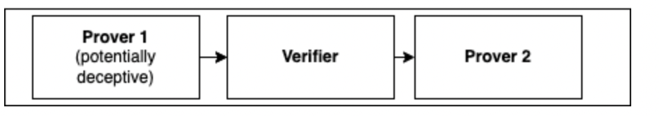
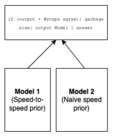
In a more general setting, we can imagine taking our task $T$ and factorizing it in some way, for example via chain-of-thought prompting when dealing with language tasks. We could have a separate adversarial model attempt to factorize the tasks in more intricate ways than simply producing a prefix of a full solution. The idea is that once the tasks become simple enough, meta-learning should no longer be necessary, and under the optimization pressure of a naive speed prior the model will have a toolkit of fast algorithms to assemble when fed full versions of the task. We intend this to be an automated form of hardcoded optimization as described in the original Risks From Learned Optimization paper by adjusting the training process to remove as much meta-learning as possible. 

Appendix B: Run-time speed priors

Throughout this post, we focused on speed prior that are applied at training time, specifically to penalize models in between steps during a training process.

There could also be application of the speed prior for inspection and run-time purposes, though given our inability to distinguish non-deceptive from deceptive models, this kind of attempt would put us squarely at the bottom of the interpretability and transparency tech tree [LW · GW], namely in worst-case inspection transparency for deceptive models:

Another point worth making here is why I haven’t separated out worst-case inspection transparency for deceptive models vs. worst-case training process transparency for deceptive models there. That’s because, while technically the latter is strictly more complicated than the former, I actually think that they’re likely to be equally difficult. In particular, I suspect that the only way that we might actually have a shot at understanding worst-case properties of deceptive models is through understanding how they’re trained. That is, if our ability to understand training dynamics is good enough, we might be able to make it impossible for a deceptive model to evade us by always being able to see its planning for how to do so during training.

Nevertheless, we examine some attempts at monitoring speed to understand the difficulties and potential intractability of this regime.

Appendix B.1: Monitoring for violation of the speed prior through run-time speed variance

Thanks to Rob Ghilduta for a conversation that inspired this idea at applying speed to perform run-time detection of deceptive formation.

Our goal is to instrument models at deployment and run-time while remaining performance competitive in order to detect violations of the speed prior. In other words, when is a model veering towards simple (and possibly deceptive) solutions rather than fast solutions?

We focus on instances where there are precursors of deception. Specifically, we focus on modeling of the operators $O$.

Here is a rough sketch of what such an operationalized scheme might look like:

1. Assume our model was built in a known ML framework $F$, say PyTorch.
2. Take the lowest available primitive in $F$ (such as the implementation of weights and activation functions), and couple it to a telemetry emitter that increments a counter whenever a full pass of the model is invoked and resets whenever a new pass begins. We use this throughout as a proxy for speed. For example, we could be collecting total activation counts across the network and forwarding them to a tool like Prometheus.
   1. There are some problems with this due to CUDA optimizations, sparse representations, and other implementation details that may make it tough to get a full grip on the “lowest primitive”. 
3. During deployment, periodically task the model with simple tasks that have known fastest solutions, i.e. perform an inspection. A model that is deceptive may be “incapable of not thinking about deception at task time,” in the sense that it must continuously be monitoring the operator $O$ and the operator’s goals in order to be aware of why it is in conformance with performing the task such that it may eventually achieve its proxy goal.
   1. Because the characteristics of the operator are variable (such as the context the operator is in, their state of mind or knowledge, etc.), the model’s modeling of the operator is also variable and different inspections will yield a different number of run-time steps when completing the simple task. We would expect this to be reflected in observing a non-zero standard deviation of the number of steps taken on simple tasks as measured by the telemetry in step 2. 
   2. A model that is intently aligned (and a model that is successfully deceptive during the inspection) will not need to monitor the variable aspects of the operator or model why it wants to perform the current task, and will be fully focused on the simple task. In other words, it will achieve a zero standard deviation of the number of steps taken on simple task as measured by the telemetry in step 2.

Can you see the problem with this setup? For one, it may not be the case that total activation count is a suitable prior for speed. On the other hand, we have incentivized our model to develop a predicate for testing whether it is under inspection or not, and disable any deceptive cognition during inspection periods (i.e. switch to acting as intently aligned as a matter of runtime characteristics). There does not seem to be an effective solution to this dilemma:

1. If we lengthen the inspection period to the full deployment, then by definition we are only employing our model for known simple tasks, which defeats the point of deploying the model.
2. If we leave gaps in the inspection periods, then we are leaving room for long-term planning in the real world–such as altering input, output and monitoring channels–that defeats the monitoring scheme. 
3. If we attempt to craft inspections for which the model cannot develop effective testing predicates, then we are in the business of instantiating a direct complex adversarial scenario against a possibly deceptive model and we should expect worst-case outcomes.
   1. On the other hand, there may be simple structures that could still provably work, such as using a non-tamperable source of randomness to invoke inspection periods when the model must simultaneously perform a known simple task and a human operator must inspect the telemetry.
   2. However, this only works in the closed-system analysis. Even with the assumption of non-tamperable sources of randomness, the gaps in inspection periods are more than sufficient to quickly put us in an ELK-type scenario. 

Appendix B.2: Cryptography-based attempts at deception

In this part of the appendix, we examine some of the existing cryptography literature to identify whether there are any suitable primitives that offer low-enough performance overhead as to be suitable for deception. The original post started out as an attempt to review that literature for any tools as to how to recover a speed measure within the encrypted domain, which could have analogue to executions within a model’s latent space. 

Any employment of cryptographic techniques by inner mesa-optimizers is, needless to say, incredibly dangerous, and identifying mechanisms available to a model for employing inner cryptographic cognition could be either (a) a precursor and potential ingredient to deceptive cognition, or (b) active deceptive cognition. In particular, we want to better understand:

1. As of techniques available in 2022, can a deceptive model make use of cryptographic methods available in public literature for some or all of its deceptive cognition without possibility of detection? In particular, we assume throughout that a model has a training distribution which has already internalized its knowledge of all such known techniques in its world model.

We note the heavy dependence on the current timestamp/year. While we cannot rule out novel methods, it is still a positive data point that we can rule out propensity towards use of existing techniques. In particular, if we are able to decrease this probability, we can establish that:

2. If there are known cryptographic techniques suitable for deceptive cognition that are not available in the public literature (e.g. the sort of training data we expect to be available in language models), then to uncover them a deceptive model must be in the process of laterally accessing confidential corporate or classified systems to acquire such techniques, which is an action with a higher barrier of detection than most other available actions (and may be disfavored by planning processes) assuming those systems are secured. 

3. If there are not any cryptographic techniques suitable for deceptive cognition available anywhere, then to find and employ such techniques the model must be performing cognition on cryptographic research internally, which may be discernibly accessible to transparency techniques available at deployment.

Because the probability mass on internal use of cryptographic techniques must be distributed across one of these three probabilities, we can constrain . In particular, we will primarily be ruling out these kinds of possibilities by considering the effective overhead imposed by such techniques (and hence a run-time speed prior) and instilling a simple assumption that we are somewhere between best-case and worst-case inspection transparency [LW · GW] for models by assuming that our transparency tools can cover $p\in (0,1)$ of a model’s total operation, in the sense of reasonably accessing predicates like “is the model using cryptography here?” or “is the model reasoning about cryptography here?” 

In particular, there are several known forms of encrypting computations such that a model could hide its inner cognition using cryptography:

1. Homomorphic Encryption
   1. Fully Homomorphic Encryption (FHE): enables the performance of various types of assessment operations on the encrypted data with unbounded range.
   2. Somewhat Homomorphic Encryption (SHE): all addition and multiplication opera- tions are permissible in SHE, but with only a limited range.
   3. Partially Homomorphic Encryption (PHE): Only one form of mathematical operation on the encrypted data is permitted in the PHE scheme, such as a multiplication or addition procedure, with an unbounded range. 
2. Secret Sharing: Only relevant to coordination between deceptive agents.
3. Secure Multi-Party Computation: Only relevant to coordination between deceptive agents.
4. Differential Privacy
   1. Privacy here is a property of both the output and the computation. “This is a method of preserving the dataset’s global statistical distribution while at the same time minimizing personally identifiable information.”
   2. Enables the perturbation of a dataset to hide individual data while preserving the ability to do statistical analysis on that same dataset. 
      1. If a deceptive model were able to encode a dataset of facts, goals or other information relevant to deception and extract them using differential privacy, it could form internal knowledge representations relevant to deception that can partially be extracted out after training. 
      2. This seems unlikely to be applicable, but we can’t rule it out.

Our review concluded that all of these currently have heavy computational overheads (e.g., >2 orders of magnitude) that would most likely be captured under even a moderately effective speed prior regardless of forwarding. The inherent mixing of speed and simplicity steers away from discovering or employing these cryptographic techniques, as they are both far from simple and very slow relative to other possible algorithms. And fortunately, hiding computations “in plain sight” without the use of cryptography appears to be impossible, so deceptive artifacts like hardcoded out-of-distribution checks should be detectable in principle by strong worst-case transparency tooling. 

We list the full set of references reviewed below with some commentary:

• Techniques for computing on encrypted data in a practical system
  • The author notes that one JustGarble, one algorithm for implementing Secure Multi-Party Computation, evaluates moderate-sized garbled-circuits at an amortized cost of 23.2 cycles per gate.
  • Also note that most computation within the encrypted domain like garbled circuits or FHE requires a pseudorandom computation and a source of randomness. There could be significant benefits to reducing a model’s ability to identify obfuscated compute mechanisms by reducing its access to sources of randomness. 
  • For example, current implementations of garbled circuits depend on Oblivious Transfer, which require sources of pseudo randomness.
• How to Run Turing Machines on Encrypted Data by Shafi Goldwasser, Yael Kalai, Raluca Ada Popa, Vinod Vaikuntanatha, and Nickolai Zeldovich
  • Salient quote: “As a consequence of this modeling, evaluating an algorithm over encrypted data is as slow as the worst-case running time of that algorithm, a dire fact for many tasks.” In other words, for encrypted computations, currently an average speed prior equals a max speed prior, as the entire circuit has to be executed.
• Better Bootstrapping in Fully Homomorphic Encryption by Craig Gentry, S. Halevi, N. Smart
  • Pure fully homomorphic encryption schemes are considerably more performant when working with a modulus very close to a power of two. But still nowhere close to being competitive with computing within a plaintext domain.
• Evaluation of the Complexity of Fully Homomorphic Encryption Schemes in Implementations of Programs
  • “Fully homomorphic programs are secure yet inefficient in terms of speed and memory usage. This stems from the fact that every encrypted bit carries a certain amount of noise in it, which grows with each operation, so in order to minimize the noise and not corrupt the data, we need to perform a bootstrapping step that significantly increases the computational time.”
  • This paper also notes that computing within a fully homomorphic domain is not Turing-complete at the moment. For example, “Breadth-First Search cannot be implemented fully homomorphically” due to limitations in having to unfold the entire circuit in advance of knowing the inputs.
• Efficient Multi-Key Homomorphic Encryption with Packed Ciphertexts with Application to Oblivious Neural Network Inference
  • This paper actually trained a model in the encrypted domain, something not out of reach for powerful meta-learners. “As a benchmark, we homomorphically classify an image using a pre-trained neural network model, where input data and model are encrypted under different keys. Our implementation takes about 1.8 seconds to evaluate one convolutional layer followed by two fully connected layers on an encrypted image from the MNIST dataset.” 
• Homomorphic Encryption without Gaussian Noise by Anamaria Costache and Nigel Smart
• Towards an efficient LWE-based fully homomorphic encryption scheme by Uddipana Dowerah, Srinivasan Krishnaswamy
  • The main applicable result is that most FHE schemes require a per-gate overhead of $O\left(n^2{L}^2\right)$ where L is the multiplicative depth of the circuit. Not very friendly to a speed prior!
• Fully Homomorphic Encryption with Polylog Overhead by C. Gentry, S. Halevi, and N.P. Smart
  • This paper by Craig Gentry, the inventor of FHE, shows arbitrary circuits can be run within FHE domains using $O\left(n\text{poly}\right(\log \left(n\right)\left)\right)$ overhead in the number of gates n.  
  • Small note: I found the terminology “polylog” confusing, but apparently this is a relatively uncommon abbreviation for “some polynomial of log(n)”.

1. ^{^}

   See point #2 under “Why You Should Love the Speed Prior” in Evan’s “Musings on the Speed Prior [AF · GW]”

2. ^{^}

   Cf Chapter 7 of Introduction to the Theory of Computation M. Sipser. Course Technology, Boston, MA, Third edition, (2013). Full argument reproduced here for clarity.

3. ^{^}

   For those inclined to more mathematical sophistication, conceive of the “napkin” as a set represented by the formal disjoint union over such finite computational traces.

4. ^{^}

   This follows from a diagonalization argument.

5. ^{^}

   If the algorithm terminates then it must do so in a finite number of steps, say $n$. Then it can only read at most $n$ bits of input off its tape when conceived as a TM.

6. ^{^}

   What are some other models of computation in which thinking about the speed prior is simpler and more tangible? For example, could we impose a speed prior within the Game of Life or some other model?

7. ^{^}

   For a few concrete examples of how different algorithms can be that produce the same outputs when given the same inputs, see the survey Program-Size Versus Time Complexity, Speed-Up and Slowdown Phenomena in Small Turing Machines. Even the identity function on 2-state machines with a 2-tape alphabet can be represented in a variety of ways: “there are 1055 TMs computing the identity function, and these TMs are distributed over 12 different algorithms (i.e. TMs that take different space/time resources).”

8. ^{^}

   For the first, see Notions of Computability at Higher Type. For the second, see Notions of Computability at Higher Type II. The third article became a full book, Higher-Order Computability by Longley and Normann.

9. ^{^}

   Without loss of generality, we will be referring to “compute budget” management whenever outer searchers are limiting the run-time complexity of the inner searched algorithms in an attempt to adhere to a mixed speed + simplicity prior. This could look very different on average-speed priors for TMs than circuit size complexity, but in general it should be possible to embed the tracking within the searcher.

10. ^{^}

    In particular, this is also a problem with non-deterministic machines, for example if our meta-learner lives in the complexity class BPP, as the use of randomness may influence the order of traversal. Given that any non-deterministic algorithm may be expressed as a deterministic algorithm by encoding the source of randomness as an auxiliary input, we focus on deterministic models of computation going forward.

11. ^{^}

    Some of the formulation of this section will change if we want to admit a dovetailer for producing the final accepted solution. Similarly, there are parallel models of computation that may employ “spliterator-like” partitioning of iterators that partition the search pattern into multiple mutually compatible traversal orders over algorithms, or even establish information channels between algorithms as part of the search. We don’t consider the sequential vs parallel or the full vs partial computation (as in dovetailing) dichotomies to be central to the forwarding problem and will refrain from considering this distinction further. Feel free to chime in in the comments if you disagree with this assessment.

12. ^{^}

    For example, see Topology, domain theory and theoretical computer science.

13. ^{^}

    Without much loss of generality, we will assume that inputs to the model are MDP tasks as in the original Are Minimal Circuits Deceptive? [AF · GW]

14. ^{^}

    As we will see, this approach requires a different calculation for the speed penalty on each input. For larger batch sizes, we can choose an aggregation of the speed penalty terms, like the average of $S_j(M_i,M_{i,j}^{\prime })$ where $j$ varies over the tasks in the batch.

15. ^{^}

    Thanks to James Lucassen for critiquing this idea and pointing out several objections that follow. The biggest concern is that it is hard to be confident of whether there is a path-dependent deviation when switching loss functions that is satisfiable under the penalty terms which actually induces the intended behavior from the model. In general, we expect there to be some alteration to a model’s weights that could elicit an execution up to the subcritical node while keeping the meta-learning tree stable, but not further. This follows from a simple entropy heuristic: because in general the parameters for the model will be vastly greater than the entropy of the input task (as a bit string, for example), we should expect to be able to make many possible deviations that will preserve the same search pattern given that the task under consideration is fixed. However, because some of the penalties are so discontinuous and include terms that go to infinity, it may be hard to achieve this deviation in practice.

16. ^{^}

    As James Lucassen points out, the output won’t necessarily change at the cut point if the outer search is tracking the best outputs it has so far, and the subcritical node does not produce that output (i.e. it occurred earlier in the search and the model is falling back to it). In this case, this mechanism will scroll back further into the meta-learning tree until it hits the second-best output. To capture this, we would need to further create an inductive bias towards meta-learning trees that are monotonically better in $L_{\text{outer}}$ the further out the search goes. This could be doable with dynamic meta-learning where we can learn from failed solutions and try to incorporate some way into the next-algorithm generator to always reach for an algorithm that does better than the previous found solution, though this also seems unnatural. On a separate point, note that if the subcritical node is extensionally the same algorithm (i.e. produces the same output as the critical node, but slower), that is fine: in a successful speed prior forwarding, there may be some searches that consecutively hit the same algorithm but at different speeds. In this case, we will be penalizing the entire chain, which should still put pressure into optimizing the part of the search pattern that constitutes the chain into finding the fastest algorithm directly (i.e., placing it at the first point of the chain).

17. ^{^}

    What is the problem with such a deceptive “virtual subcritical” node if its tail section, the algorithm that returns, is always the true fastest solution for the task? It seems the deceptive portion of the algorithm hasn’t accomplished much since it must adhere rigorously to the speed penalty and the task in order to output. Well, for one, ensuring this condition holds out of distribution is very hard due to conditional defection [LW · GW], such as by installing a check for factorizability of RSA-2048. 

18. ^{^}

    There is one more obvious idea: in this particular case, we would like to be able to variate the meta-learning tree rather than keep it constant (for example, by relaxing the computational signature penalty mentioned earlier to allow several different tree structures as we compute $L_{\text{inner}}$), as a priori we would expect different structures could locate the same fastest algorithm but run into different deceptive inner algorithms that would have a very difficult time acausally communicating in a way that isn’t detectable. For example, if there was a natural Schelling point at which to install the decoy cut point across different deceptive algorithms that emerge from different meta-learning tree structures and hence search patterns for the same task input, then we should be able to compute that point as well and raise a massive warning flag whenever it occurs as the value of the critical node speed. Alas, the natural Schelling point is the true run-time of the fastest algorithm for solving the task. Embedding a variant of “return Y,” where Y is a valid solution, but with additional garbage logic to land at the right run-time – should suffice. We can still hold out hope that the inner algorithms reach different values for the estimated fastness, but this is probably a losing battle.

5 comments

Comments sorted by top scores.