Magna Alta Doctrina

post by jacob_cannell · 2021-12-11T21:54:36.192Z · LW · GW · 7 comments

Contents

  Introduction: a Reckoning
  Preliminaries
  Foundations
  Deep Factoring
  Who art thou calling a Local optimizer
  Doing the good Rev. Bayes' work
  Behold, a Mighty Cannon of Glass
    Model Drift / Parameter Staleness
    Variance and Normalization
    Variance and Learning Rate
    Orthogonality, Sparsity, Compression, and Learning
  Solomonoff Networks and EGD
  Conclusions
None
7 comments

Continuing topics from an earlier 2015 blog post, The Brain as a Universal Learning Machine [LW · GW], this new series will begin with updated distillations of deep learning's best learnings, then interweave brain (reverse)engineering, advanced simulation tech, crypto-economic mechanism design, and more, interject a bit of novelty, then future project those intertwined threads into an ambitious systemic proto-plan for a new research economy to build advanced sims and aligned AGI. The telic ambition of this sequence - on it's best boldest days - is to evolve into that plan; or if failing that, at least engage as futurism.

This sequence will explore answers to three intertwined key questions:

1. How can we build powerful scalable predictive world models?
2. How can we efficiently plan/steer/optimize the future using said models?
3. How can we best ensure said powerful optimization is aligned to our values?

These problems and their solutions are not wholly distinct, but rather deeply interconnect in a fractal recurrence. But before exploring that, first we must establish common knowledge of the foundations, and before that: a quick reckoning.

Introduction: a Reckoning

“Having been trained as a computer scientist in the 90s, everybody knew that AI didn’t work. People tried it, they tried neural nets and none of it worked.”

-Sergey Brin, Davos 2017

Few foresaw the Connectivist's [LW · GW] sudden sweeping victory. Why?

In this post I will reveal and explore the key foundations of Deep Learning's success. And reveal is the correct word; some of these insights are rare even within the field. I will argue that these insights predict/postdict the success of DL, and towards the end I will venture further to argue that any practical AGI will necessarily be built on a DL-like foundation (regardless of map nomenclature), and perhaps stake on that with some novel predictions.

In a popular AI textbook from a bit before the DL revolution (the Norvig/Russell one), I recall a chapter discussing Artificial Neural Networks as a technique near a chapter on Evolutionary Computation, perhaps nearby chapters labeled Bayesian Inference or Decision Trees, and all the other separated magisteria. The chapter on ANNs made sure to point out how they only did marginally better than SVMs (support vector machines) on key benchmarks like MNIST at the time, despite being far less theoretically sound (which should only make them more interesting - for what then explained that extra bit of success?). This is how the popular textbook(s) mapped the terra incognita algorithmica before the DL revolution: with ANNs as just one peculiar, unpromising and oddly shaped tool in a large technical toolbox of competing techniques. The influence of this mindset still persists today due to inertia.

In contrast the Connectivist mindset is holistic rather than reductionist, reverent of seemingly messy biology and neuroscience over crisp formalism, pragmatic and experimental over theoretical, philosophically inspired by integrative systems theory, cybernetics and AI futurists such as Moravec/Kurzweil who claimed/predicted (decades in advance) that hardware was the main constraint and thus AGI would arrive fairly predictably at the end of the Moore's Law rainbow (ie early 2020's), when brain level compute finally became available for cheap PC prices. Key to the Connectivist mindset are the two distinct but correlated beliefs that biological brains are both effective practical implementations of intelligence, and that reverse engineering the brain is tractable because it's complexity is an emergent evolutionary phenomenon arising from the interaction of the information environment and surprisingly simple universal learning algorithms. As a result Connectivists tend to envision a more anthropomorphic AGI. 

The principle opponent of Connectivism - it's opposite direction in mindspace -  I will name Formalism: a primarily reductionist mindset, reverent of the crisp purity of mathematics and formal proofs, infatuated with the evolved modularity hypothesis, dismissive of the ugly messy biological brain with all it's attendant cognitive biases and irrationality, and thus relatively assured that AGI would not, should not, come from reverse engineering the brain, no more than flying machines arrived [LW · GW] from reverse engineering the flapping wings of birds, or submarines derived from fish, or automobiles from horses. To the Formalists, anthropomorphizing [LW · GW] AGI is a grave cognitive sin [? · GW].

Now to be fair, defining the Formalist position as the exact opposite of Connectivism is perhaps arguably a strawman. These clusters are rough categorizations, like principle components in belief-space. Few individuals strongly hold all the exact beliefs in the cluster as I defined them, and some formalists would argue that they agree(d) that intelligence may reduce to simple algorithms. 

But ultimately the proof is in the predictive pudding. Few/none in the formalist camp demonstrably predicted that the requisite simple learning algorithms were already mostly discovered/proposed long ago and merely needed to be refined and scaled up, or that the brain's complexity was likewise emergent from simple universal learning, or that if you put a human brain in a dolphin's environment, it could automatically learn the complex sensory modality of echolocation. The connectivist viewpoint implicitly predicted the winning paradigm for AI, as DL is simply it's direct descendant. The connectivist futurists even mostly-correctly predicted the timing of connectivism's victory, and (in my case apparently) predicted [LW(p) · GW(p)] the year of AlphaGo five years in advance, as just a few random examples.

We clearly now live in the Connectivist/DL future; the zeitgeist of the field is updating, and even though the larger scale debate [LW(p) · GW(p)] over the road to AGI rages on, it is increasingly intra-paradigm rather than inter-paradigm.

The holistic approach of Connectivism, as in literally connecting all useful paradigms, as evident in deep learning's evolutionary history as a cross fertilizing integration of best techniques from diverse fields: bayesian graphical modeling, neuroscience, traditional optimization, GOFAI, etc, indicates that the mental framing of disparate competing techniques was itself misguided: not even wrong.

Preliminaries

Traditional computing is built on the foundation of the boolean algebra: minimal binary variables {0,1} and logic operations {eg: AND,OR,NOT}, which we directly realize in hardware using some minimal universal logic gate family. A CPU is essentially an interpreter burnt into circuit-form to implement a more complex and powerful 32-bit or 64-bit assembly language, and modern programming languages then build an even more useful/productive type and operator algebra on top that core foundation.

Deep learning - ie neural nets - are currently implemented on that foundation through simulation, but they are not of that foundation. Neural networks are circuits built from the real tensor algebra: the algebra built from matrices/tensors of real numbers and a small library of intrinsically parallel tensor operators (eg: multiplication, addition, a few element-wise non-linearities, etc). Binary circuits have binary connections; an edge is either present or absent.  Neural networks replace binary edges with  more flexible weighted edges, or edge probabilities. This lifting to the real algebra allows smooth interpolations across circuit space and thus full circuit inference using continuous optimization methods (ie gradient descent). 

Rather than program a system directly, in the DL paradigm your code instead describes an informal prior or abstract rough high level plan for a circuit architecture. A neural circuit designer don't need to know the messy details of how the circuit truly works in the way actual circuit engineers do (this in particular infuriates [LW · GW] formalists). Instead you apply a powerful optimizer (eg SGD, more realistically Adam or newer variants) to infer or carve out an effective circuit which is fully implied by - and indirectly specified by - the data observed subject to the constraints of the architectural prior. In that sense DL is the scruffier, more practical, and far more successful sibling of the lesser known Probabilistic Programming paradigm which augments traditional programming languages with direct programmer specified uncertainty over functions which is then reduced through some approximate bayesian inference or optimization process.

Perhaps counter-intuitively, much of the best new results in DL come from specifying less rather than more.  Armed with a powerful optimizer, one can often progress simply by removing expert knowledge instilled into architectural priors that inadvertently incorrectly constrain optimization rather than guide it to success. 

To an outside observer (or a recalcitrant unreformed formalist), deep learning has much the appearance of algorithmic alchemy: simply add more layers to whatever model people are tweeting about, carefully feed it a huge dataset under the watchful supervision of overpaid ML engineers, make sure to hit the monetize! button before the competition, and then rejoice/retire in a big heap pile of utility.

The pragmatic reality for anyone who has actually built their own DL engines and models from scratch is perhaps worse: when SGD/bprop works it is almost magical, but it can tragically fail just as mysteriously. Predicting why it works - for certain combinations of model components, optimizers, hyperparams, and environments - seems very much like experimental sorcery. And sometimes even it's mysterious successes can be annoying: on several occasions serious, seemingly-critical bugs in one of my custom matmul codes were mostly rerouted over by SGD, resulting only in a modest drop in predictive accuracy. But insert some new operator or change an innocuous-seeming hyper parameter and suddenly training explodes. 

This inexorably led me to search out deeper core intuitions. A significant portion of DL research papers consist of arguably random tweaks to prior successful models: grad student descent writ large, but fortunately, buried within and throughout the great arxiv-straining-heap that is modern DL, there are actual foundational insights that can help explain/predict in advance which altered rituals and recipes will likely succeed.

Foundations

The core problem in DL/ML, or just intelligence in general - presenting in myriad variations - is that of statistical inference: finding high likelihood solutions conditioned on input data/observations. Inference is closely related to optimization; a fully general solution to one of these paradigms can also solve the other. Optimization is the process of finding high value configurations, so any inference problem can be solved by optimizing for posterior probability (ie truth). Going the other direction we can often redefine truth as value (tilting a probability distribution into a value distribution - implied by the word 'loss' function), and reframe optimization as inference. 

An exact in-theory computable solution to the algorithmic inference problem was proposed all the way back in 1960 by Ray Solomonoff. You are probably already familiar [LW · GW] with Solomonoff Induction, so I will only briefly recap.

The key principle is to assign a prior distribution over the space of all program-models using a formalization of Occam's razor (minimum description length), and then infer the posterior distribution over all of model-space using Bayes' rule:

$p\left(h|E\right)=\frac{p\left(E|h\right)L(h{)}^{-1}}{p\left(E\right)}$

Where $p\left(E|h\right)$ - the probability of the evidence given the program-model h - is simply 1 if h has successfully predicted all evidence/observations, or 0 otherwise. The prior, $L(h{)}^{-1}$, is simply the inverse program length, in some universal encoding: a simple measure of complexity. Notice the denominator - the evidence prior $p\left(E\right)$ - is a normalization constant that doesn't depend on h, and can be ignored in many inference scenarios where we are just interested in the relative likelihoods of things.

Given this theoretically computable posterior distribution over all program-models that could explain the data, we can then make optimal predictions by 'simply' computing a weighted average of the predictions from each program-model $h$ in $H$, weighted by their current cumulative posterior $p\left(h|E\right)$ (normalization is already performed in the posterior computation):

$p\left(e\right)={\sum }_{h\in H}p\left(h|E\right)p\left(e|h\right)$

Where p(e|h) is the predictive output of h for the next observation e. In machine learning terms, Solomonoff induction predicts using the universal ensemble: the ensemble of all computable models.

The choice of Occam's razor for the prior over functions is also well justified. Assuming the observations were in fact generated from some unknown computable function, there are also (infinitely) many distractor functions that just happen to contain and output the correct observation prefix without modelling anything, with frequency of such distractors increasing exponentially with program complexity, which the Occam penalty thus helps adjust for.

Given a powerful general inference engine (efficient approximation to universal inference), there are several obvious ways we could use that to construct powerful AGI:

1. Mesa: We use the inference engine in the inner loop of a planning search/optimizer to infer actions with high long term (discounted) expected utility
2. Meta: We employ the inference engine to explore deep simulations which contain high utility architectures within.

AIXI is a pure theoretical example of a direct type 1 mesa solution (ignoring any practical compute constraints), whereas Deepmind's EfficientZero [LW · GW] agent is a more practical and important recent example.

However EZ's lineage was evolved in sims and is thus arguably a type-2 example. All useful type-2 meta solutions will implicitly contain type-1 mesa solutions internally (and likewise type-1 solutions often contain deep sims internally ...), thus these two approaches are more complementary components of an interleaved recursion rather than fully competing and distinct techniques.

Deep Factoring

Obviously full bayesian inference ala Solomonoff - implemented directly - is infeasible as it requires time exponential in program size. But can we do asymptotically better using something like dynamic programming approximation? Well, yes! And this is one of the core foundational secrets of DL's success.

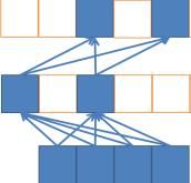
Consider a stacked 'deep' network of width W and depth D, where W >= $2^D$, with a minimal sparse connectivity such that each node has a fan-in of 2, and an additional final output on top. Such a network can simultaneously in parallel encode and evaluate at most W sub-functions, where each sub-function is equivalent to a parse-tree like program of length ~ $2^D$(the binary tree expanding down from a single node in the top hidden layer), but the total cost of evaluation is only polynomial: ~$D{W}^2$ or $2DW$ rather than $2^{D}W$.  ($2DW$ if fully exploiting max sparsity in the connectivity matrix, potentially even less with full sparsity in both matrices) 

How is this possible? Because all of these functions are fully sharing/reusing subcomputations. Full program space is highly redundant; with many partial function duplicates that share internal structure. The term 'deep factoring' is my own, but I may have acquired the insight while reading the 2011 sum-product networks paper (still worth a read today): they explain it in terms of computable probability distributions and don't name the concept as such, but it's equivalent.

So just by converting to circuit form and using the then obvious evaluation method for circuit form, you can search over an exponential slice of program/circuit space in polynomial time. The caveat is that this is inherently perhaps a somewhat biased sampling of program space, and with increasing depth comes increasing optimization complexity, but in practice those are fair prices to pay for exponential speedup.

I still occasionally hear some say "Neural networks are just a fad, there will be other paradigms", or "We'll find some other better approximation to Bayes/Solomonoff inference/induction", but no, because: deep factoring . It's possible that AGI will arrive later than I anticipate such that there will be a new marketing term that replaces "Deep Learning", but even in those rare worlds, make no mistake: deep factoring is essential.

Deep factoring isn't so useful now as a predictive insight simply because DL has already taken over. But consider that not all once-popular paradigms exploit this insight: most evolutionary computing and program search techniques for example, generally do not happen to structure computations in just the right way so as to take advantage of deep factoring.

Designing and thinking in the circuit form paradigm also has another tremendous practical advantage: it brings one much intimately closer to the hardware physics and thus makes GPU parallelization much easier (and by 'GPU' I more generally mean all relevant full parallel processor tech past dennard scaling).

Who art thou calling a Local optimizer

A very common misconception of DL/GD is that it is a purely local search method. A local search method is one that maintains a single promising candidate solution which is adjusted through small incremental improvements (ie approximate bayesian updates) after observing/updating on each input datum. Think of a single ball rolling around a loss landscape. Now DL - if restrictively defined for a second as ANNs+SGD - would be strictly local if it was somehow constrained to use a circuit no larger than the solution circuit, but it is most definitely not so constrained.

Take whatever circuit structure you had in mind as the solution candidate, then just copy paste it and merge to get a new dual circuit that is twice as wide and equivalent to evaluating two variations of the original circuit simultaneously - rinse and repeat as needed. And as I just explained in the previous section, with deep factoring we can also do better by using some mix of width and depth, exploring a large space of candidate sub-circuits simultaneously in parallel. Then with appropriate sparsity and exploration techniques, we can do even better still by exploring a much larger solution space over time rather than limiting ourselves to only the memory constrained spatial dimension.

This all should have been very obvious to everyone from the start, but large overcomplete deep nets can automatically implement complex parallel hill climbing type optimization over internal ensembles (a swarm of balls rolling around exploring the landscape, sharing internal sub-computations). Overcomplete deep nets laugh in glee at formalists as they steamroll over local minima.

And even though this should have been obvious, there is now an entire little sub-branch of DL exploring the apparently-surprising idea of finding winning subnetworks embedded in a larger overcomplete network: the 'lottery ticket hypothesis', a research thread in DL that does connect to the crucial topic of sparsity, which I'll discuss in more depth later.

Over-completeness is part of the explanation of why SGD can generalize so well, but it's not sufficient on it's own: we still need to explain how/why big overcomplete ANNs can internally approximate parallel hill climbing with a swarm of regularized sub-solutions rather than just massively overfit.

There is an obvious way to construct a neural layer that does explicit Bayes/Solmonoff style ensembling, which I'll explore towards the end, but standard DL systems don't do that in any obvious way and yet still can strongly generalize, so we need a more general explanation. 

Doing the good Rev. Bayes' work

If GD/SGD is doing inference, and useful probabilistic inference is always in some fashion an approximation to Bayesian inference - what's the connection? How so? 

Let us begin by gazing intently at what GD actually is/does, in simple form:

${\theta }^{\prime }=\theta -\alpha \frac{\partial L\left(f_{\theta }\right(x\left)\right)}{\partial \theta }$

Where $x$ is an input to our model function $f$ parameterized by params $\theta$. This defines the SGD/GD parameter update (learning) rule as a small step in the gradient direction of decreasing loss, which alternatively could be defined as:

${\theta }^{\prime }=\alpha \frac{\partial U\left(f_{\theta }\right(x\left)\right)}{\partial \theta }+\theta$

Where U is utility. (ie equating loss to negative utility)

This slight rearrangement also makes the connection to bayesian inference a bit more explicitly clear: the gradient update is an approximation to the likelihood component of the bayesian posterior update, and the sampled model parameters are parameter distribution means, all in log-probability form (so that multiplication becomes addition).

$log\left(p\right(\theta |f_{\theta }\left(x\right))=log(p\left(f_{\theta }\right(x\left)|\theta \right))+log(p\left(\theta \right))$

In the DL setting, each input $x$ typically corresponds to a single/few observation(s) from some huge set, and thus provides only a small amount of update evidence. The learning rate $\alpha$ is a heuristic approximation to the correct ratio of current update vs all previous (encapsulated in the prior). We'll soon derive a more explicit connection between proper bayesian informed learning rates and precision/variance/uncertainty with non-trivial implications.

Notice the above bayesian-ish posterior omits the evidence prior - the normalizing denominator - and thus computes an unnormalized distribution. This is fine if we are only concerned with sampling the promising parameters, but forgoes the ability to compute absolute posterior probability estimates. GD is then even more constrained in that it uses a locally linear approximation and is thus only informing us about the relative merits of a tiny close region in parameter space.  

As we are typically using an implied utility distribution (through a loss function which translates/interprets utility as probability), this means that GD can help us find valuable posterior parameter configurations, but it doesn't tell us anything about the true absolute expected utility values of any parameters or configurations. Using an economic analogy, GD would be the equivalent of backpropagating detailed notes for myriad tiny design changes back through supply chains, without backpropping any absolute price (utility) information. This is unfortunate because it turns out that efficient execution is a form of economic reasoning which works best with absolute utility estimates to determine which computations are actually valuable, a topic I'll eventually return to with connections to sparsity and shapley values.

The loss gradient defines a unique direction to move in parameter space that maximizes a form of local efficiency measure: maximizing loss/utility change per unit parameter magnitude - ie entropy. There are many other possible directions one could move in (and a landscape of more complex algorithms for choosing such directions), and for almost all systems of interest, the specific direction GD uses is not that which leads most directly to the goal of a global minima or strong local minima.

For a simple intuitive example, consider an optimization landscape in the shape of a not quite flat plane which is ever so slightly tilted to the right. One could stroll leisurely to the right for a very long time for ever decreasing loss. Now add a small but steep local indention right near the current position in parameter space. GD, being greedy, will gleefully choose to dive into that local minima, instead of taking the slower gradual path that leads to much lower long term loss. Other optimizers - such as 2nd order optimizers (we'll explore more in a bit) - will in this situation choose the longer path to lower loss, and in fact can often move with arbitrary quickness down gentle graded slopes.

Nonetheless, for most complex problems of interest, GD is often wise to greedily choose myopic quick-to-compute small improvements over large farsighted jumps to potentially lower loss. Why?

Because by economizing through the path of minimal efficient effort, GD ensures that it isn't moving too far in parameter space into the vast region of overfitting. There is an infinite space of complexity expanding out with distance from the origin, with ever increasing more tempting lower minima, but the farther one goes from the low complexity origin the more likely these are false non-generalizing solutions, prone to overfitting. A good init for GD is a low complexity init, and GD indirectly penalizes or avoids moving quickly away from the low complexity origin.

Then on top of that form of intrinsic regularization, one also typically employs one or more regularizers - such as a direct penalty on weight magnitude/complexity. These regularizers act like a gravitational force pulling GD trajectories towards the low complexity origin, further ensuring it approximately explores solutions with a proper Solomonoff/Occam complexity tradeoff (and naturally more farsighted alternatives generally must use such regularization to avoid overfitting).

In practice in the online setting we care about we are most always using stochastic gradient descent - which adds a bit of implicit noise that further helps bounce out of local minima at the expense of increased variance which generally slows convergence but is reduced through momentum and or batching. Unless otherwise noted, I use GD to mean SGD, implied by default.  

Ideal training of overcomplete ANNs with GD and proper normalization has three (not always temporarily distinct) phases:

• An initial phase of disappointment
• A learning phase progressing eventually to low/zero test error (overfitting)
• A hidden 2nd continued learning phase eventually leading to low validation error (generalization) - ie grokking

However in practice GD can be finnicky and brittle: it seems very difficult to predict in advance which combinations of architectures, techniques, optimizers, hyperparams, etc allow GD to actually work rather than just explode.

Behold, a Mighty Cannon of Glass

In this admittedly verbose section, I'll attempt to demystify GD and distill insights into the nature of the it's approximation to full bayesian inference, what approximation assumptions cause GD to fail when violated, and what has/can be done about it.

Let's begin with a minimal network layer computing: $f\left(x\right)=\varphi \left(Wx\right)$, with input vector $x$ of dim Nx1 and weight matrix W of dim KxN, and some activation function $\varphi$.  We'll then add a simple loss function on the output,  the quadratic loss with target y of dim K:  

$L\left(f\right(x\left)\right)=(y-f(x){)}^2:f(x)=\varphi (Wx)$

Notice we could then recursively expand in depth or time by recursive substitution of $x=f\left(x^{\prime }\right)$, ie $f\left(x\right)=\varphi \left(W\varphi \right(W{x}^{\prime }\left)\right)$, so this simple model is still fully universal in potential.    

However, GD makes the key simplifying assumption of local linearity: it optimizes a local linear approximation to the true function. We will start first with just the linearity assumption, which is equivalent for our purpose to removing the non-linear activation functions from consideration in the joint log likelihood, ie:

$L\left(f\right(x\left)\right)\approx (y-f^{\prime }(x){)}^2:f^{\prime }(x)=Wx$

Given this simplification, we now focus on the surprising remaining complexity of a single linear layer.  For even after this linearity assumption/simplification, an analysis to derive the implied posterior reveals important insights into both the problem structure and GD's weaknesses, requires only basic algebra, and should be considered table stakes for deeper understanding of deep learning.

This quadratic loss function describes how well the function $f\left(x\right)$ does as a generator/predictor when fed input $x$, compared to the (posthoc) target output $y$: ie a training target (or perhaps backpropagated target for hidden layers).

The bayesian view of the loss/utility function is that the predictive loss is describing a log probability distribution (or rather an unnormalized reshaped expected utility distribution). Working in log probability space simplifies products of normal distributions down to addition of polynomials.

Our loss function here outputs a scalar which we'll now interpret as the total log probability of observing output y given input x and our model output $f\left(x\right)$:

$L\left(f\right(x\left)\right)=log\left(p\right(y|f\left(x\right)\left)\right)=(y-f(x){)}^2$

 $p\left(y|f\right(x\left)\right)=e^{(y-f(x){)}^2}$

So Bayes informs us that the quadratic loss corresponds to the modeling assumption of a normal distribution for the predictive error (in log probability space), minus a few irrelevant scaling constants and the suspicious absence of a variance term (assumption of unit variance). Adding a predictive variance component could allow this model to also predict and 'price in' it's own uncertainty, but we'll leave out that potentially-quite-useful component for now.

Solomonoff induction is full bayesian inference over binary functions, but here we are using real valued circuits - and assuming the normal distribution is justified - we are still well within the bayesian inference paradigm. 

Notice that in log space the normal distribution is just a 2nd order polynomial:

$(\frac{x-u_x}{v_x}{)}^2=\frac{1}{v_x^2}{x}^2+(-2\frac{u_x}{v_x^2})x+\frac{u_x^2}{v_x^2}$

$=a{x}^2+bx+c:a=\frac{1}{v_x^2},b=-2\frac{u_x}{v_x^2},c=\frac{u_x^2}{v_x^2}$

$v_x^2=\frac{1}{a},u_x=-\frac{1}{2}{v}_x^{2}b=-\frac{1}{2}\frac{b}{a}$

Since the log of products corresponds to the sum of their logs (multiplication/divison is addition/subtraction in log-space):

log(x*y) = log(x)+log(y)

Thus the product of normal distributions in log space is simply the sum of their polynomials (from here on I will abbreviate $log\left(p\right(x\left)\right)$ as $lp\left(x\right)$ ):

$lp\left(x|e\right)=lp\left(\right(e|x\left)p\right(x\left)\right)=(a_{e|x}+a_x)x^2+(b_{e|x}+b_x)x+c_{e|x}+c_x$

$a_{x|e}{x}^2+b_{x|e}x+c_{x|e}=(a_{e|x}+a_x)x^2+(b_{e|x}+b_x)x+c_{e|x}+c_x$

So we can later just add in more polynomial terms for our priors to get a full joint posterior (ignoring the evidence prior normalization factor for now). With that background, let's return to our example:

$L\left(f\right(x\left)\right)=lp\left(y|f\right(x\left)\right)=(y-f(x){)}^2=(y-Wx{)}^2:f\left(x\right)=Wx$

$lp\left(y|f\right(x\left)\right)=\left(Wx\right)\cdot \left(Wx\right)+(-2y)\cdot Wx+y\cdot y$

$lp\left(y|f\right(x\left)\right)=x^{T}Zx-2y^{T}Wx+y^{T}y:Z=W^{T}W$

$lp\left(y|f\right(x\left)\right)=(x^{T}Z-2y^{T}W)x+y^{T}y:Z=W^{T}W$

In a slight customization/abuse of notation, I will use $x_i$ to describe the sparse vector formed from setting all entries in x other than i to zero (ie selecting i), and then $x_{/i}$ to describe the inverse: the vector formed from setting only entry i to zero (removing i).

We can isolate for a single x variable to get it's quadratic-form:

$lp\left(y|f\right(x_i\left)\right)=W_{ii}^2{x}_i^2+(x_{/i}^{T}Z-2y^{T}W)x_i:Z=W^{T}W$

The 1st order term for $x_i$ has a loss increasing component, $x_{/i}^{T}Z$, and a loss decreasing component,  $-2y^{T}W$. The latter component $-2y^{T}W$ measures how increasing hidden node $x_i$ decreases the loss proportional to $x_i$'s output effect: the dot product of $x_i$'s fanout vector and the target y.  If the network outputs images, then y would be a prediction image target, and $x_i$'s fanout vector (column in W), would be it's learned image feature component, so their dot product measures the rate of loss decrease by increasing the value of $x_i$ (activating that neuron). 

Z is an interference matrix completely determined from the connection matrix W, it captures the 2nd order interactions: the cosine similarity between the fan-out connectivity vectors for each pair of nodes in x.  Each entry $z_{ij}\in Z$ measures the similarity or redundancy in output effect between all the outgoing connections of nodes $x_i$ and $x_j$.

If two nodes $x_i$ and $x_j$ happened to be perfectly redundant (fanout dot product of 1), then solving for the optimal value of each in isolation would fail - it would result in an output exactly 2x too large. If Z happens to be the identity matrix, that indicates that the fan-out connectivity vectors for each node in x (column in W) are completely orthogonal. In that unrealistic ideal scenario, then the interference term $x^{T}Z$ would be a minimal diagonal matrix, and $x_{/i}^{T}Z$ would be zero. The diagonal of  $x^{T}Z$ corresponds to the variance or L2-mag of each x's fanout weight vector, or just 1 if W is normalized - I separate out this component as $W_{ii}^2{x}_i^2$ for $x_i$ in the equation above. 

In the scenario where  $x_{/i}^{T}Z$ is a zero matrix (through some combination of sparsity or orthogonality in W), then we can reduce to a simpler scalar quadratic equation:

$lp\left(y|f\right(x_i\left)\right)=W_{ii}^2{x}_i^2-2y^{T}W{x}_i$

With $a=W_{ii}^2,b=-2y^{T}W$

Standard 1st order backprop instead uses a local 1st order (linear) taylor approximation of the system, which we can write out as a pertubation:

$lp\left(y|f\right(x\left)\right)\approx (y-f(x_0)-f(x_{\Delta }){)}^2$

$lp\left(y|f\right(x_{\Delta }\left)\right)=(y_{\Delta }-f(x_{\Delta }){)}^2:y_{\Delta }=y-f(x_0)$

Notice $y_{\Delta }$ is the difference between the target and the function output, ie the bprop gradient.

$lp\left(y|f\right(x_{\Delta i}\left)\right)=W_{ii}^2{x}_{\Delta i}^2+(x_{\Delta /i}^{T}Z-2y_{\Delta }^{T}W)x_{\Delta i}:Z=W^{T}W$

And again if $x_{\Delta /i}^{T}Z$ is zero:

$lp\left(y|f\right(x_{\Delta i}\left)\right)=W_{ii}^2{x}_{\Delta i}^2-2y_{\Delta }^{T}W{x}_{\Delta i}$

Vanilla GD/bprop then uses only the 1st order $b$ term and simply ignores the 2nd order $a$ term of the implied quadratic (although some optimizers such as Adam post-hoc estimate a 2nd order term). This 1st order approximation is reasonably justified because of the linear system approximation, as long as we are taking sufficiently small steps such that the higher order terms don't dominate - and thus constrains convergence/learning speed.  

Because we already assumed a linear approximation to the system, stacking additional layer depth or unrolling in time remains linear, it doesn't lead to increasingly high order polynomial complexity.

Now back to our full posterior and 2nd order analysis:

$lp\left(f\right(x\left)|y\right))=lp(y|f\left(x\right))+lp(f\left(x\right)\left)\right)$

The prior for our function on the right side is our distribution over parameters before observing the new evidence, and - for simplicity/efficiency - can be modeled as a product of independent component normal distributions for each parameter (ignoring constants):

$lp\left(f\right(x\left)\right)=lp\left(W\right)+lp\left(X\right)=A_{W_0}\cdot W\circ W+B_{W_0}\cdot W+A_{W_0}\cdot X\circ X+B_{X_0}\cdot X$

Now, to simplify analysis, let's look at the special case where our tensors X,W are of dimension 1, ie scalars.

Combining the prior and loss likelihood into a posterior:

$lp\left(f\right(x\left)|y\right)=lp\left(y|f\right(x\left)\right)+lp\left(f\right(x\left)\right)$

$lp\left(y|f\right(x\left)\right)+lp\left(f\right(x\left)\right)=w^2{x}^2+(-2y)wx+y^2+a_{w_0}{w}^2+b_{w_0}w+a_{x_0}{x}^2+b_{x_0}x$

This equation describes the total posterior (unnormalized) log-probability as a function of all variables. Now we can rearrange and isolate terms to get a posterior over only w:

$lp\left(w|y\right)=(x^2+a_{w_0})w^2+(b_{w_0}-2yx)w$

And then converting back from quadratic form to normal/gaussian form:

$v_{w|y}^2=\frac{1}{x^2+a_{w_0}},u_{w|y}=\frac{1}{2}\frac{2yx-b_{w_0}}{x^2+a_{w_0}}$

Or for a sequence of updates (replacing y with Y) :

$lp\left(w|Y\right)=(x_0^2+x_1^2...+a_{w_0})w^2+(b_{w_0}-2(y_0{x}_0+y_1{x}_1...\left)\right)w$

$u_{w|Y}=\frac{y_0{x}_0+z_1{x}_1...-\frac{1}{2}{b}_{w_0}}{x_0^2+x_1^2...+a_{w_0}}$

Notice that if the two components of the prior: $b_{w_0}$ and $a_{w_0}$ are 0, then our derived posterior mean of w is just $u_{w|z}=z/x$ for the single scalar case, which is just what you'd expect, as that is the value which generates the output: $z=wx$.

Now let's focus on how the mean of w updated:

$\Delta u_w=u_{w|y}-u_w=\frac{(2yx-b_{w_0})}{2x^2+2a_{w_0}}-\frac{-b_{w_0}}{2a_{w_0}}$

Notice that the update is proportional to z, and roughly inversely proportional to x and the prior precision $a_{w_0}$:

$\Delta u_w\propto \frac{z}{x{a}_{w_0}}\propto \frac{v_w^{2}z}{x}$

So our derived update through a multiplication operator here is directly inverting the multiplication (seemingly the inverse of gradient descent), but also notice crucially that the relative variance/precision (ratio of likelihood-update precision to prior precision) is very much like a learning rate scale.

As discussed earlier, GD doesn't attempt to jump immediately to the best solution (even if that is obviously correct and possible in this simple case).  If one wants the target output of w*x to be 1, and x is currently 0.001, then the most reasonable guess for w (or updates of w) is on order 1000, not 0.001 - but that implies an enormous (and thus highly improbable when assuming normally distributed) value for w.

In scenarios with wild variation in scale, GD does in fact trip on it's face. Consider tracing a gradient through f(x) = a*b*x, where parameter a is 100, parameter b is 0.0001, and both x and the loss are on order 1. GD will update a on order 0.0001, update b on order 100, pass down updates on order 0.01 to x, and then ... rapidly explode.

In other words, gradient descent only works reliably in the unit variance regime - standard GD assumes unit variance. And in that regime it works quite well, because it moves in the direction of minimal efficient effort. As discussed earlier, it does not move directly in the direction that would minimize steps towards the goal, but instead moves in the direction that maximizes progress towards the goal per unit entropy (as entropy is proportional to weight magnitude).

So what can we postdict from this? In summary here are some interesting findings:

Model Drift / Parameter Staleness

The posterior over parameters is the final product of the prior and all evidence updates throughout the entire learning process. However as we are only maintaining a single point/mean estimate of all the parameters which will change significantly during training, this implies that older updates are actually incorrect as they were computed with a different configuration, with the approximation error generally increasing with age as the network drifts away from the specific historical parameter state a particular older update was computed with. As the computed update loses approximation validity as you move away from that point in parameter space, this suggests that we should somehow slowly forget/erase the effect of older updates. This is exactly what weight decay helps with: weight decay helps correct for parameter drift - in addition to acting like a regularizer. And indeed if there wasn't a need to adjust for parameter/update drift, then arguably weight decay wouldn't be required, as the bayesian prior could be encoded purely in the initial weight distribution.

Variance and Normalization

In general SGD will fall flat on it's face if we don't carefully ensure unit variance. So armed with this knowledge, if you went back in time to just 8 years ago, you could predict the importance and success of various forms of normalization like batch normalization (32k citations and counting), or normalization of layers, groups, or weights. Or perhaps you could have derived something like the Adam optimizer (90k+ citations!) which roughly estimates the first 2 moments through slow temporal statistics and then computes the mean parameter estimate by taking the $a/b$ ratio similar to the derived rule above.

A while ago as a little experiment I derived and implemented a method that backprops local 2nd order polynomials directly, rather than roughly estimating them using slow moving averages ala Adam. It uses 2x as much RAM and roughly 2x compute vs 1st order GD, but in theory avoids all normalization difficulties (as the variance is now more properly estimated and dynamically tracked through computations). I only ever got around to testing it on small toy problems, where it worked well, but haven't bothered to try scaling it up yet. It would probably need explicit regularization to avoid overfitting. I found later that my 'bprop2' is similar in spirit to, but lighter weight than, Path-sgd, although with other key differences, and the derivation is quite different. These methods are obviously related to 2nd order optimization algorithms, although those are usually working with more complex higher order gradient curvature approximations. (If time permits, I'll also explore the 2nd order interaction terms, and how they connect to sparse coding and brain inhibitory circuits).

Variance and Learning Rate

The simple bayesian analysis of our linear system suggests a deep connection between precision/variance and ideal learning rates which properly balance updates. Recall after each update step the new mean is:

$u_{x|e}=-\frac{1}{2}\frac{b_{e|x}+b_x}{a_{e|x}+a_x}$

Parameters generally should start with a low precision prior $a_x$ (high variance) with precision increasing after each update resulting in an inverse power law decrease in learning rate, although ideally we should be more directly approximating the precision/variance of updates themselves. Weight decay would then counteract this by decaying $a_x$ back to it's default or 0, tempering the power law falloff to more linear and potentially resulting in a more complex learning rate schedule.

Proper tracking of 2nd order precision/variance could probably also help with the key problem of catastrophic forgetting (if not just outright solve it), when combined with sparsity. As we accumulate enough solid evidence ($a_x$ getting large enough) the learning rate on that parameter slows to a crawl to preserve information.  However there is always some reserve of unused/underused connections (ala sparisity) with low precision $a_x$ values which can change rapidly.

And this indeed is exactly what we see in the brain, with a wide variety of implied learning rates: the equivalent precision/variance of synaptic connections runs the full gamut from a small core of long term stable connections down to a sea of smaller undetermined synapses that are in flux on the timescale of seconds, and everything in between.

A precision of 0 (variance inf) implies a learning rate of 0: absolute certainty that a particular connection should not exist. In some subsequent post, I will explore the idea that a major failing of current DL results from using an implied prior precision of 0 on implied large-scale architectural connectivity (which prevents SGD from learning large scale architecture directly), rather than assigning reasonable non-zero priors and applying SGD to everything for full scale meta-architecture meta-learning (and indeed if you look in the brain, there are clearly distinct modules with mostly local connectivity which is a direct-from-physics constraint, but nonetheless there are also widely dispersed weak connections at all levels).

Orthogonality, Sparsity, Compression, and Learning

Perhaps the deepest lesson from our simple analysis is hidden in the interference matrix term:

$(x_{/i}^{T}Z-2y^{T}W)x_i:Z=W^{T}W$

The interference matrix constrains the maximal viable learning rate/speed: inference is easy/fast when Z is close to the identity matrix and/or x is sparse. In the case where $x_i$ is a 1-hot vector (a single nonzero), then $x_i^{\prime }$s outgoing weights - the fanout vector $W_i$ - can absorb the entirety of the error update (learning rate near 1). Naturally a 1-hot vector may be too computationally impoverished and limiting, but we can keep adding nonzeros to x and maintain the maximal learning rate as long as each new $x_j$ is completely orthogonal and has an independent error reducing effect on y. Sparse outgoing connectivity in W naturally also helps with this independence/orthogonality, and generally will correlate with sparsity in x (the hidden state).

We should also carefully notice when occam's razor - our complexity penalty prior - can apply just as much to our hidden state activation x as it does to the long term connectivity weights W.  If our network is a vision system for example, then overfitting in the weights would cause the obvious symptoms of memorizing overly specific patterns and failure to generalize. However, the network can also potentially overfit it's internal temporary representations it uses to model sensory observations, leading to brittle representations that are overly sensitive to - and fail to filter out - noise and thus are susceptible to adversarial examples.

Imposing a low complexity prior on our hidden state activations - uniformly or at least at key bottlenecks - can be considered a powerful unsupervised learning prior all by itself. In fact, one of the key building blocks of modern DL - the relu activation function - originates from  "Deep Sparse Rectifier Networks", which besides fulfilling the DL trifecta of sexy appeal to performance, theory, and neuroscience-inspiration, references and is inspired by the previous sparse coding literature, a sort of unsupervised proto-DL without much deepness (contemporary to Hinton's boltzmann machines).

Sparse coding in essence seeks to approximate the general linear target reconstruction type objective $(y-Wx{)}^2$ we analyzed earlier, combined with an L0 or L1 prior on the hidden activation state $x$ to induce sparse activations.  Solving these equations then usually involves a bilevel optimization with an inner inference loop over the sparse $x$ codes for a specific example/image, and a slower outer inference loop (usually using SGD) to learn the filters/weights W.  With the correct sparsity prior and settings the solutions will learn cortex like gabor features that intrinsically compress and are immediately useful for many low level image tasks (such as denoising).

However this bilevel optimization is naturally expensive, leading to several faster approximations - one of  the more popular of which was ISTA (Iterative Shrinking Thresholding Algorithm) - which essentially is an iterative relu network with a small negative bias. Then Gregor/LecCun showed you could quickly approximate the inner iteration of algorithms like ISTA with a fairly shallow ANN, leading into the current stacked relu paradigm, as especially exemplified in the popular resnet architecture, which in fact learns stacked layers of unrolled iterative estimators, like a stacked unrolled ISTA.

There are interesting tradeoffs between sparsity, capacity, and the spectrum between fast memoization and slow generalization. Consider a simple two layer network with a large linear hidden layer followed by a sparsification step (k-max, sparse coding, etc), and a linear output layer. A sparse activation layer with a single nonzero (1-hot) is essentially equivalent to encoding a memory address. The forward pass then first performs a pattern match in the first layer, comparing the input to all stored patterns to compute the closest match as an address for a memory lookup in the second output layer (with optional linear scaling).  The maximal backprop update through that maximally sparse hidden layer corresponds to simply remembering the current input and output patterns, ie it corresponds rather directly to a memory write. 

As you increase the number of nonzeros to relax sparsity in the hidden layer, the backprop update diffuses the stored pattern across more rows of the matrix (more features), rather than concentrating into a single clear memory access. This eventually could allow for greater generalization, but slows down learning in proportion, requiring more data to converge to something useful. It should be clear that there is no one optimal type of memory representation - and AGI will probably employ a continuous spectrum across the sparsity/capacity space, perhaps with successive re-encoding as more data becomes available. We see at least one level of this in the brain, where episodic memory is first stored in a very sparse fast memory system in the hippocampus/top-center cortex, and then later slowly migrates down to lower cortex during sleep memory consolidation.

So purely by controlling sparsity and learning rates in a generic RNN, one could implement various forms of short or medium term memory systems - ie one could emulate transformers which employ a short term sequence memory (see this paper for another perhaps more complex/clunky equivalence between transformers and fast weights).

Where is this all going? The current main research track in DL descends in part from a particular fork from the unsupervised sparse coding stream which - after switching to relus - mostly ignored activation sparsity because the GPU codes everyone uses (provided by nvidia) don't provide any speedup advantage for sparsity. However, when/if that changes, expect major leaps in performance (both runtime and convergence) from previously underexplored branches of this research tree. 

 

Solomonoff Networks and EGD

In the previous section I explored how GD/SGD is a powerful form of approximate bayesian inference, with some key caveats such as the implicit assumption of normal distributions, unit variance, local linearity, etc.

Assuming normal distributions is quite reasonable for semi-linear networks that are built out of matrix multiplication and minimally non-linear functions such as the piece-wise linear relu. The output accumulation of matrix multiplication will be normally distributed via central limit for addition, and the relu non-linearity will convert to a rectified gaussian which is arguably optimal if your goal is to maintain normal distribution as much as possible.

But might it be limiting to only assume additive combinations and normal distributions? If we go back and look at what Solomonoff induction does, it doesn't look much like GD at the surface level. If we converted solomonoff induction to network form with a single output node with N inputs, each input would represent a different sub-model function. The output is computed as just the standard weighted sum, but the weight update rule would be quite different.

In the most direct mapping the update rule would simply prune to 0 the connection to every input sub-model which failed to predict an output, doing that after each observation: Solomonoff throws away half the theory space at every step. The real weight value is then just the complexity penalty. In an ANN implementation with a sparse connectivity constraint we could enforce an approximately uniform complexity of all sub-models, and thus use only binary connection weights.  The practical form of this would then prune half the connections at every step, and then reclaim that valuable circuit space by growing new random connections.

While that approach is potentially interesting by itself, it's probably better to stay within the real algebra. The Solmonoff style partial continuous update for real-valued weights would then correspond to a multiplicative weight update rather than an additive weight update as in standard SGD.

Has this been tried/evaluated? Why actually yes - it's called exponentiated gradient descent, as exponentiating the result of additive updates is equivalent to multiplicative updates. And intriguingly, for certain 'sparse' input distributions the convergence or total error of EGD/MGD is logarithmic rather than the typical inverse polynomial of AGD (additive gradient descent): $O\left(logN\right)$ vs $O\left(1/N\right)$ or $O\left(1/N^2\right)$, and fits naturally with 'throw away half the theories per observation'.

The situations where EGD outperforms AGD, or vice versa, depend on the input distribution: if it's more normal then AGD wins, if it's more sparse log-normal then EGD wins. The morale of the story is there isn't one single simple update rule that always maximizes convergence/performance; it all depends on the data distribution (a key insight from bayesian analysis).

The exponential/multiplicative update is correct in Solomonoff's use case because the different sub-models are strictly competing rather than cooperating: we assume a single correct theory can explain the data, and predict through an ensemble of sub-models. But we should expect that learned cooperation is also important - and more specifically if you look more deeply down the layers of a deeply factored net at where nodes representing sub-computations are more heavily shared, it perhaps argues for cooperative components.

A practical quirk of multiplicative/exponential udpates is they imply non-negativity (as the exp(x) is always positive), so you have to add extra terms and work to get negative weights.

What about replacing additive operations in the forward pass with multiplicative interactions?  Instead of ${\sum }_{i=1}^N{w}_i{x}_i$, how about ${\prod }_{i=1}^N{w}_i{x}_i$?  In practice all we need to do is use a log activation function in one layer followed by exp activation function in the next to convert from linear/additive space to exponential/multiplicative space: no changes to the matrix multiplication code required. Surely someone has tried that? Well the top google result is a blog post which seems interesting, but alas no experiment. 

Multiplicative layers with log/exp alternating activation functions may be difficult to train (and indeed this suggests one should use EGD or at least exp(w) reparameterization), but they seem promising for automatically learning fast softmax style competitive normalization groups, and more generally for multiplicative gating.  They could also directly implement a form of transformer-style attention for example.  

So it's probably no coincidence that if we look in the brain we see primarily multiplicative synapse updates, non-negative weights (negative connections implemented through dedicated interneurons with inhibitory neurotransmitters), some multiplicative neuron interactions (ie inhibitory axon gating), and a general pattern of log-normal statistics rather than normal.

Conclusions

Deep learning is swallowing up ML/AI research and investment into it's fold like some black hole attractor, accelerating us towards AGI. It's success ultimately derives from the conjuncture of efficient flexible approximations to bayesian inference from above and the constraints of physics from below. There is still tremendous work to be done, but the DL path to AGI is quickly coalescing into clarity. I am concerned that the end times approach, but also hopeful/optimistic that we still have an opportunity to steer the outcome.  

Now that I've covered some of the foundational preliminaries, in subsequent posts I'll explore the fun stuff (not necessarily in this order):

• The latest developments in mind/brain reverse engineering, possibly as part of a rough historical comparison of brain-evolution's 10^9 year timeline vs DL/tech evolution's 10^2 year timeline, and the implications for AGI
• An exploration of how DL will transform computer graphics leading to Matrix quality simulations, and derived insights into scaling both AGI world models and planning
• A more comprehensive technical proposal for massively scaling up fully sparse meta-architecture meta-learning to address the current weaknesses in DL (parts of this arguably should be time-lock censored)
• A deeper focused dive into Azathoth [LW · GW]'s approximate solution to the value-learning problem: the evolution of altruism/empathy/love etc, the surprisingly simple key lessons, and their implications for inner alignment.
• A discussion of future socio-economic structures: how fast approximations to shapley values and various prediction/decision markets could change everything, mechanism design, social orgs as agents, and the implications for outer alignment; leading to a sketch of a future superintelligence as a crypto-economic governance system, backpropagating it's immense future value through time into the present to bootstrap itself into existence.

 

 

 

7 comments

Comments sorted by top scores.