Finite Factored Sets
post by Scott Garrabrant · 2021-05-23T20:52:48.575Z · LW · GW · 95 commentsContents
  1. Short Combinatorics Talk
    1m. Some Context
    1t. Factoring the Talk
    1b. Set Partitions
    1b. Set Factorizations
    1e. Enumerating Factorizations
  2. The Main Talk (It's About Time)
    2m. The Pearlian Paradigm
    2t. We Can Do Better
    2b. Time and Orthogonality
    2e. Game of Life
    2b. Conditional Orthogonality
    2b. Compositional Semigraphoid Axioms
    2b. The Fundamental Theorem
    2b. Temporal Inference
    2e. Two Binary Variables (Pearl)
    2e. Two Binary Variables (Factored Sets)
    2b. Applications / Future Work / Speculation
None
97 comments
This is the edited transcript of a talk introducing finite factored sets. For most readers, it will probably be the best starting point for learning about factored sets.
Video:
(Lightly edited) slides: https://intelligence.org/files/Factored-Set-Slides.pdf
1. Short Combinatorics Talk
1m.
Scott: So I want to start with some context. For people who are not already familiar with my work:
- My main motivation is to reduce existential risk.
- I try to do this by trying to figure out how to align advanced artificial intelligence.
- I try to do this by trying to become less confused about intelligence and optimization and agency and various things in that cluster.
- My main strategy here is to develop a theory of agents that are embedded [? · GW] in the environment that they're optimizing. I think there are a lot of open hard problems around doing this.
- This leads me to do a bunch of weird math and philosophy. This talk is going to be an example of some weird math and philosophy.
For people who are already familiar with my work, I just want to say that according to my personal aesthetics, the subject of this talk is about as exciting as Logical Induction, which is to say I'm really excited about it. And I'm really excited about this audience; I'm excited to give this talk right now.
1t.
This talk can be split into 2 parts:
- Part 1: a short pure-math combinatorics talk.
I suspect that if I were better, I would instead be giving a short pure-math category theory talk; but I'm trained as a combinatorialist, so I'm giving a combinatorics talk upfront.
- Part 2: a more applied and philosophical main talk.
This talk can also be split into 4 parts differentiated by color: , , , and . Combining these gives us 8 parts (some of which are not contiguous):
| Part 1: Short Talk | Part 2: The Main Talk | |
| 1m. Some Context [LW · GW] | 2m. The Pearlian Paradigm [LW · GW] | |
| 1t. Factoring the Talk [LW · GW] | 2t. We Can Do Better [LW · GW] | |
| 1b. Set Partitions [LW · GW], etc. | 2b. Time and Orthogonality [LW · GW], etc. | |
| 1e. Enumerating Factorizations [LW · GW] | 2e. Game of Life [LW · GW], etc. |
1b.
All right. Here's some background math:
- A partition of a set is a set of non-empty subsets of , called parts, such that for each there exists a unique part in that contains .
- Basically, a partition of is a way to view as a disjoint union. We have parts that are disjoint from each other, and they union together to form .
- We'll write for the set of all partitions of S.
- We'll say that a partition is trivial if it has exactly one part.
- We'll use bracket notation, , to denote the unique part in containing . So this is like the equivalence class of a given element.
- And we'll use the notation to say that two elements and are in the same part in .
You can also think of partitions as being like variables on your set . Viewed in that way, the values of a partition correspond to which part an element is in.
Or you can think of as a question that you could ask about a generic element of . If I have an element of and it's hidden from you and you want to ask a question about it, each possible question corresponds to a partition that splits up according to the different possible answers.
We're also going to use the lattice structure of partitions:
- We'll say that ( is finer than , and is coarser than ) if makes all of the distinctions that makes (and possibly some more distinctions), i.e., if for all , implies . You can break your set into parts, , and then break it into smaller parts, .
- (the common refinement of and ) is the coarsest partition that is finer than both and . This is the unique partition that makes all of the distinctions that either or makes, and no other distinctions. This is well-defined, which I'm not going to show here.
Hopefully this is mostly background. Now I want to show something new.
1b.
A factorization of a set is a set of nontrivial partitions of , called factors, such that for each way of choosing one part from each factor in , there exists a unique element of in the intersection of those parts.
So this is maybe a little bit dense. My short tagline of this is: "A factorization of is a way to view as a product, in the exact same way that a partition was a way to view as a disjoint union."
If you take one definition away from this first talk, it should be the definition of factorization. I'll try to explain it from a bunch of different angles to help communicate the concept.
If is a factorization of , then there exists a bijection between and given by . This bijection comes from sending an element of to the tuple consisting only of parts containing that element. And as a consequence of this bijection, .
So we're really viewing as a product of these individual factors, with no additional structure.
Although we won't prove this here, something else you can verify about factorizations is that all of the parts in a factor have to be of the same size.
We'll write for the set of all factorizations of , and we'll say that a finite factored set is a pair , where is a finite set and .
Note that the relationship between and is somewhat loopy. If I want to define a factored set, there are two strategies I could use. I could first introduce the , and break it into factors. Alternatively, I could first introduce the . Any time I have a finite collection of finite sets , I can take their product and thereby produce an , modulo the degenerate case where some of the sets are empty. So can just be the product of a finite collection of arbitrary finite sets.
To my eye, this notion of factorization is extremely natural. It's basically the multiplicative analog of a set partition. And I really want to push that point, so here's another attempt to push that point:
| A partition is a set of of such that the obvious function the of the elements of is a bijection. | A factorization is a set of of such that the obvious function the of the elements of is a bijection. |
I can take a slightly modified version of the partition definition from before and dualize a whole bunch of the words, and get out the set factorization definition.
Hopefully you're now kind of convinced that this is an extremely natural notion.
Andrew Critch: Scott, in one sense, you're treating "subset" as dual to partition, which I think is valid. And then in another sense, you're treating "factorization" as dual to partition. Those are both valid, but maybe it's worth talking about the two kinds of duality. Scott: Yeah. I think what's going on there is that there are two ways to view a partition. You can view a partition as "that which is dual to a subset," and you can also view a partition as something that is built up out of subsets. These two different views do different things when you dualize. Ramana Kumar: I was just going to check: You said you can start with an arbitrary and then build the from it. It can be literally any set, and then there's always an ... Scott: If none of them are empty, yes, you could just take a collection of sets that are kind of arbitrary elements. And you can take their product, and you can identify with each of the elements of a set the subset of the product that projects on to that element. Ramana Kumar: Ah. So the in that case will just be tuples. Scott: That's right. Brendan Fong: Scott, given a set, I find it very easy to come up with partitions. But I find it less easy to come up with factorizations. Do you have any tricks for...? Scott: For that, I should probably just go on to the examples. Joseph Hirsh: Can I ask one more thing before you do that? You allow factors to have one element in them? Scott: I said "nontrivial," which means it does not have one element. Joseph Hirsh: "Nontrivial" means "not have one element, and not have no elements"? Scott: No, the empty set has a partition (with no parts), and I will call that nontrivial. But the empty set thing is not that critical. |
I'm now going to move on to some examples.
1e.
Exercise! What are the factorizations of the set ?
Spoiler space:
.
.
.
.
.
.
.
.
.
.
First, we're going to have a kind of trivial factorization:
We only have one factor, and that factor is the discrete partition. You can do this for any set, as long as your set has at least two elements.
Recall that in the definition of factorization, we wanted that for each way of choosing one part from each factor, we had a unique element in the intersection of those parts. Since we only have one factor here, satisfying the definition just requires that for each way of choosing one part from the discrete partition, there exists a unique element that is in that part.
And then we want some less trivial factorizations. In order to have a factorization, we're going to need some partitions. And the product of the cardinalities of our partitions are going to have to equal the cardinality of our set , which is 4.
The only way to express 4 as a nontrivial product is to express it as . Thus we're looking for factorizations that have 2 factors, where each factor has 2 parts.
We noted earlier that all of the parts in a factor have to be of the same size. So we're looking for 2 partitions that each break our 4-element set into 2 sets of size 2.
So if I'm going to have a factorization of that isn't this trivial one, I'm going to have to pick 2 partitions of my 4-element set that each break the set into 2 parts of size 2. And there are 3 partitions of a 4-element sets that break it up into 2 parts of size 2. For each way of choosing a pair of these 3 partitions, I'm going to get a factorization.
So there will be 4 factorizations of a 4-element set.
In general you can ask, "How many factorizations are there of a finite set of size ?". Here's a little chart showing the answer for :
| 0 | 1 |
| 1 | 1 |
| 2 | 1 |
| 3 | 1 |
| 4 | 4 |
| 5 | 1 |
| 6 | 61 |
| 7 | 1 |
| 8 | 1681 |
| 9 | 5041 |
| 10 | 15121 |
| 11 | 1 |
| 12 | 13638241 |
| 13 | 1 |
| 14 | 8648641 |
| 15 | 1816214401 |
| 16 | 181880899201 |
| 17 | 1 |
| 18 | 45951781075201 |
| 19 | 1 |
| 20 | 3379365788198401 |
| 21 | 1689515283456001 |
| 22 | 14079294028801 |
| 23 | 1 |
| 24 | 4454857103544668620801 |
| 25 | 538583682060103680001 |
You'll notice that if is prime, there will be a single factorization, which hopefully makes sense. This is the factorization that only has one factor.
A very surprising fact to me is that this sequence did not show up on OEIS, which is this database that combinatorialists use to check whether or not their sequence has been studied before, and to see connections to other sequences.
To me, this just feels like the multiplicative version of the Bell numbers. The Bell numbers count how many partitions there are of a set of size . It's sequence number 110 on OEIS out of over 300,000; and this sequence just doesn't show up at all, even when I tweak it and delete the degenerate cases and so on.
I am very confused by this fact. To me, factorizations seem like an extremely natural concept, and it seems to me like it hasn't really been studied before.
This is the end of my short combinatorics talk.
Ramana Kumar: If you're willing to do it, I'd appreciate just stepping through one of the examples of the factorizations and the definition, because this is pretty new to me. Scott: Yeah. Let's go through the first nontrivial factorization of : In the definition, I said a factorization should be a set of partitions such that for each way of choosing one part from each of the partitions, there will be a unique element in the intersection of those parts. Here, I have a partition that's separating the small numbers from the large numbers: . And I also have a partition that's separating the even numbers from the odd numbers: . And the point is that for each way of choosing either "small" or "large" and also choosing "even" or "odd", there will be a unique element of that is the conjunction of these two choices. In the other two nontrivial factorizations, I replace either "small and large" or "even and odd" with an "inner and outer" distinction. David Spivak: For partitions and for many things, if I know the partitions of a set and the partitions of a set , then I know some partitions of (the disjoint union) or I know some partitions of . Do you know any facts like that for factorizations? Scott: Yeah. If I have two factored sets, I can get a factored set over their product, which sort of disjoint-unions the two collections of factors. For the additive thing, you're not going to get anything like that because prime sets don't have any nontrivial factorizations. |
All right. I think I'm going to move on to the main talk.
2. The Main Talk (It's About Time)
2m.
We can't talk about time without talking about Pearlian causal inference [? · GW]. I want to start by saying that I think the Pearlian paradigm is great. This buys me some crackpot points, but I'll say it's the best thing to happen to our understanding of time since Einstein.
I'm not going to go into all the details of Pearl's paradigm here. My talk will not be technically dependent on it; it's here for motivation.
Given a collection of variables and a joint probability distribution over those variables, Pearl can infer causal/temporal relationships between the variables. (In this talk I'm going to use "causal" and "temporal" interchangeably, though there may be more interesting things to say here philosophically.)
Pearl can infer temporal data from statistical data, which is going against the adage that "correlation does not imply causation." It's like Pearl is taking the combinatorial structure of your correlation and using that to infer causation, which I think is just really great.
Ramana Kumar: I may be wrong, but I think this is false. Or I think that that's not all Pearl needs—just the joint distribution over the variables. Doesn't he also make use of intervention distributions? Scott: In the theory that is described in chapter two of the book Causality, he's not really using other stuff. Pearl builds up this bigger theory elsewhere. But you have some strong ability, maybe assuming simplicity or whatever (but not assuming you have access to extra information), to take a collection of variables and a joint distribution over those variables, and infer causation from correlation. Andrew Critch: Ramana, it depends a lot on the structure of the underlying causal graph. For some causal graphs, you can actually recover them uniquely with no interventions. And only assumptions with zero-measure exceptions are needed, which is really strong. Ramana Kumar: Right, but then the information you're using is the graph. Andrew Critch: No, you're not. Just the joint distribution. Ramana Kumar: Oh, okay. Sorry, go ahead. Andrew Critch: There exist causal graphs with the property that if nature is generated by that graph and you don't know it, and then you look at the joint distribution, you will infer with probability 1 that nature was generated by that graph, without having done any interventions. Ramana Kumar: Got it. That makes sense. Thanks. Scott: Cool. |
I am going to (a little bit) go against this, though. I'm going to claim that Pearl is kind of cheating when making this inference. The thing I want to point out is that in the sentence "Given a collection of variables and a joint probability distribution over those variables, Pearl can infer causal/temporal relationships between the variables.", the words "Given a collection of variables" are actually hiding a lot of the work.
The emphasis is usually put on the joint probability distribution, but Pearl is not inferring temporal data from statistical data alone. He is inferring temporal data from statistical data and factorization data: how the world is broken up into these variables.
I claim that this issue is also entangled with a failure to adequately handle abstraction and determinism. To point at that a little bit, one could do something like say:
"Well, what if I take the variables that I'm given in a Pearlian problem and I just forget that structure? I can just take the product of all of these variables that I'm given, and consider the space of all partitions on that product of variables that I'm given; and each one of those partitions will be its own variable. And then I can try to do Pearlian causal inference on this big set of all the variables that I get by forgetting the structure of variables that were given to me."
And the problem is that when you do that, you have a bunch of things that are deterministic functions of each other, and you can't actually infer stuff using the Pearlian paradigm.
So in my view, this cheating is very entangled with the fact that Pearl's paradigm isn't great for handling abstraction and determinism.
2t.
The main thing we'll do in this talk is we're going to introduce an alternative to Pearl that does not rely on factorization data, and that therefore works better with abstraction and determinism.
Where Pearl was given a collection of variables, we are going to just consider all partitions of a given set. Where Pearl infers a directed acyclic graph, we're going to infer a finite factored set.
In the Pearlian world, we can look at the graph and read off properties of time and orthogonality/independence. A directed path between nodes corresponds to one node being before the other, and two nodes are independent if they have no common ancestor. Similarly, in our world, we will be able to read time and orthogonality off of a finite factored set.
(Orthogonality and independence are pretty similar. I'll use the word "orthogonality" when I'm talking about a combinatorial notion, and I'll use "independence" when I'm talking about a probabilistic notion.)
In the Pearlian world, d-separation, which you can read off of the graph, corresponds to conditional independence in all probability distributions that you can put on the graph. We're going to have a fundamental theorem that will say basically the same thing: conditional orthogonality corresponds to conditional independence in all probability distributions that we can put on our factored set.
In the Pearlian world, d-separation will satisfy the compositional graphoid axioms. In our world, we're just going to satisfy the compositional semigraphoid axioms. The fifth graphoid axiom is one that I claim you shouldn't have even wanted in the first place.
Pearl does causal inference. We're going to talk about how to do temporal inference using this new paradigm, and infer some very basic temporal facts that Pearl's approach can't. (Note that Pearl can also sometimes infer temporal relations that we can't—but only, from our point of view, because Pearl is making additional factorization assumptions.)
And then we'll talk about a bunch of applications.
| Pearl | This Talk |
| A Given Collection of Variables | All Partitions of a Given Set [LW · GW] |
| Directed Acyclic Graph | Finite Factored Set [LW · GW] |
| Directed Path Between Nodes | "Time" [LW · GW] |
| No Common Ancestor | "Orthogonality" [LW · GW] |
| d-Separation | "Conditional Orthogonality" [LW · GW] |
| Compositional Graphoid | Compositional Semigraphoid [LW · GW] |
| d-Separation ↔ Conditional Independence | The Fundamental Theorem [LW · GW] |
| Causal Inference | Temporal Inference [LW · GW] |
| Many Many Applications | Many Many Applications [LW · GW] |
Excluding the motivation, table of contents, and example sections, this table also serves as an outline of the two talks. We've already talked about set partitions and finite factored sets, so now we're going to talk about time and orthogonality.
2b.
I think that if you capture one definition from this second part of the talk, it should be this one. Given a finite factored set as context, we're going to define the history of a partition.
Let be a finite factored set. And let be partitions of .
The history of , written , is the smallest set of factors such that for all , if for all , then .
The history of , then, is the smallest set of factors —so, the smallest subset of —such that if I take an element of and I hide it from you, and you want to know which part in it is in, it suffices for me to tell you which part it is in within each of the factors in .
So the history is a set of factors of , and knowing the values of all the factors in is sufficient to know the value of , or to know which part in a given element is going to be in. I'll give an example soon that will maybe make this a little more clear.
We're then going to define time from history. We'll say that is weakly before , written , if . And we'll say that is strictly before , written , if .
One analogy one could draw is that these histories are like the past light cones of a point in spacetime. When one point is before another point, then the backwards light cone of the earlier point is going to be a subset of the backwards light cone of the later point. This helps show why "before" can be like a subset relation.
We're also going to define orthogonality from history. We'll say that two partitions and are orthogonal, written , if their histories are disjoint: .
Now I'm going to go through an example.
2e.
Let be the set of all Game of Life computations starting from an board.
Let (i.e., cells computable from the initial board). For , let be the set of all computations such that the cell at row and column is alive at time .
(Minor footnote: I've done some small tricks here in order to deal with the fact that the Game of Life is normally played on an infinite board. We want to deal with the finite case, and we don't want to worry about boundary conditions, so we're only going to look at the cells that are uniquely determined by the initial board. This means that the board will shrink over time, but this won't matter for our example.)
is the set of all Game of Life computations, but since the Game of Life is deterministic, the set of all computations is in bijective correspondence with the set of all initial conditions. So , the number of initial board states.
This also gives us a nice factorization on the set of all Game of Life computations. For each cell, there's a partition that separates out the Game of Life computations in which that cell is alive at time 0 from the ones where it's dead at time 0. Our factorization, then, will be a set of binary factors, one for each question of "Was this cell alive or dead at time 0?".
Formally: For , let . Let , where .
There will also be other partitions on this set of all Game of Life computations that we can talk about. For example, you can take a cell and a time and say, "Is this cell alive at time ?", and there will be a partition that separates out the computations where that cell is alive at time from the computations where it's dead at time .
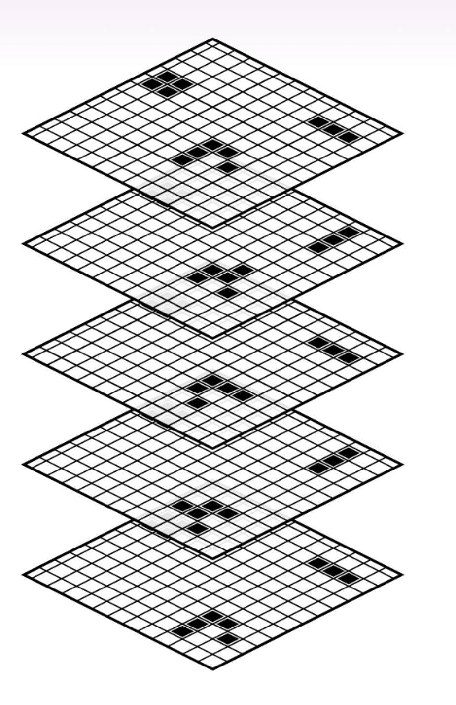
Here's an example of that:
The lowest grid shows a section of the initial board state.
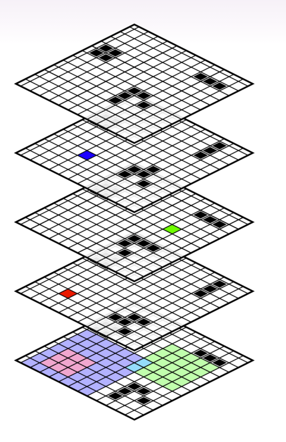
The blue, green, and red squares on the upper boards are (cell, time) pairs. Each square corresponds to a partition of the set of all Game of Life computations, "Is that cell alive or dead at the given time ?"
The history of that partition is going to be all the cells in the initial board that go into computing whether the cell is alive or dead at time . It's everything involved in figuring out that cell's state. E.g., knowing the state of the nine light-red cells in the initial board always tells you the state of the red cell in the second board.
In this example, the partition corresponding to the red cell's state is strictly before the partition corresponding to the blue cell. The question of whether the red cell is alive or dead is before the question of whether the blue cell is alive or dead.
Meanwhile, the question of whether the red cell is alive or dead is going to be orthogonal to the question of whether the green cell is alive or dead.
And the question of whether the blue cell is alive or dead is not going to be orthogonal to the question of whether the green cell is alive or dead, because they intersect on the cyan cells.
Generalizing the point, fix , where . Then:
- .
- if and only if and .
- if and only if or .
We can also see that the blue and green cells look almost orthogonal. If we condition on the values of the two cyan cells in the intersection of their histories, then the blue and green partitions become orthogonal. That's what we're going to discuss next.
David Spivak: A priori, that would be a gigantic computation—to be able to tell me that you understand the factorization structure of that Game of Life. So what intuition are you using to be able to make that claim, that it has the kind of factorization structure you're implying there? Scott: So, I've defined the factorization structure. David Spivak: You gave us a certain factorization already. So somehow you have a very good intuition about history, I guess. Maybe that's what I'm asking about. Scott: Yeah. So, if I didn't give you the factorization, there's this obnoxious number of factorizations that you could put on the set here. And then for the history, the intuition I'm using is: "What do I need to know in order to compute this value?" I actually went through and I made little gadgets in Game of Life to make sure I was right here, that every single cell actually could in some situations affect the cells in question. But yeah, the intuition that I'm working from is mostly about the information in the computation. It's "Can I construct a situation where if only I knew this fact, I would be able to compute what this value is? And if I can't, then it can take two different values." David Spivak: Okay. I think deriving that intuition from the definition is something I'm missing, but I don't know if we have time to go through that. Scott: Yeah, I think I'm not going to here. |
2b.
So, just to set your expectations: Every time I explain Pearlian causal inference to someone, they say that d-separation is the thing they can't remember. d-separation is a much more complicated concept than "directed paths between nodes" and "nodes without any common ancestors" in Pearl; and similarly, conditional orthogonality will be much more complicated than time and orthogonality in our paradigm. Though I do think that conditional orthogonality has a much simpler and nicer definition than d-separation.
We'll begin with the definition of conditional history. We again have a fixed finite set as our context. Let be a finite factored set, let , and let .
The conditional history of given , written , is the smallest set of factors satisfying the following two conditions:
- For all , if for all , then .
- For all and , if for all and for all , then .
The first condition is much like the condition we had in our definition of history, except we're going to make the assumption that we're in . So the first condition is: if all you know about an object is that it's in , and you want to know which part it's in within , it suffices for me to tell you which part it's in within each factor in the history .
Our second condition is not actually going to mention . It's going to be a relationship between and . And it says that if you want to figure out whether an element of is in , it's sufficient to parallelize and ask two questions:
- "If I only look at the values of the factors in , is 'this point is in ' compatible with that information?"
- "If I only look at the values of the factors in , is 'this point is in ' compatible with that information?"
If both of these questions return "yes", then the point has to be in .
I am not going to give an intuition about why this needs to be a part of the definition. I will say that without this second condition, conditional history would not even be well-defined, because it wouldn't be closed under intersection. And so I wouldn't be able to take the smallest set of factors in the subset ordering.
Instead of justifying this definition by explaining the intuitions behind it, I'm going to justify it by using it and appealing to its consequences.
We're going to use conditional history to define conditional orthogonality, just like we used history to define orthogonality. We say that and are orthogonal given , written , if the history of given is disjoint from the history of given : .
We say and are orthogonal given , written , if for all . So what it means to be orthogonal given a partition is just to be orthogonal given each individual way that the partition might be, each individual part in that partition.
I've been working with this for a while and it feels pretty natural to me, but I don't have a good way to push the naturalness of this condition. So again, I instead want to appeal to the consequences.
2b.
Conditional orthogonality satisfies the compositional semigraphoid axioms, which means finite factored sets are pretty well-behaved. Let be a finite factored set, and let be partitions of . Then:
- If , then . (symmetry)
- If , then and . (decomposition)
- If , then . (weak union)
- If and , then . (contraction)
- If and If , then . (composition)
The first four properties here make up the semigraphoid axioms, slightly modified because I'm working with partitions rather than sets of variables, so union is replaced with common refinement. There's another graphoid axiom which we're not going to satisfy; but I argue that we don't want to satisfy it, because it doesn't play well with determinism.
The fifth property here, composition, is maybe one of the most unintuitive, because it's not exactly satisfied by probabilistic independence.
Decomposition and composition act like converses of each other. Together, conditioning on throughout, they say that is orthogonal to both and if and only if is orthogonal to the common refinement of and .
2b.
In addition to being well-behaved, I also want to show that conditional orthogonality is pretty powerful. The way I want to do this is by showing that conditional orthogonality exactly corresponds to conditional independence in all probability distributions you can put on your finite factored set. Thus, much like d-separation in the Pearlian picture, conditional orthogonality can be thought of as a combinatorial version of probabilistic independence.
A probability distribution on a finite factored set is a probability distribution on that can be thought of as coming from a bunch of independent probability distributions on each of the factors in . So for all .
This effectively means that your probability distribution factors the same way your set factors: the probability of any given element is the product of the probabilities of each of the individual parts that it's in within each factor.
The fundamental theorem of finite factored sets says: Let be a finite factored set, and let be partitions of . Then if and only if for all probability distributions on , and all , , and , we have . I.e., is orthogonal to given if and only conditional independence is satisfied across all probability distributions.
This theorem, for me, was a little nontrivial to prove. I had to go through defining certain polynomials associated with the subsets, and then dealing with unique factorization in the space of these polynomials; I think the proof was eight pages or something.
The fundamental theorem allows us to infer orthogonality data from probabilistic data. If I have some empirical distribution, or I have some Bayesian distribution, I can use that to infer some orthogonality data. (We could also imagine orthogonality data coming from other sources.) And then we can use this orthogonality data to get temporal data.
So next, we're going to talk about how to get temporal data from orthogonality data.
2b.
We're going to start with a finite set , which is our sample space.
One naive thing that you might think we would try to do is infer a factorization of . We're not going to do that because that's going to be too restrictive. We want to allow for to maybe hide some information from us, for there to be some latent structure and such.
There may be some situations that are distinct without being distinct in . So instead, we're going to infer a factored set model of : some other set , and a factorization of , and a function from to .
A model of is a pair , where is a finite factored set and . ( need not be injective or surjective.)
Then if I have a partition of , I can send this partition backwards across and get a unique partition of . If , then is given by .
Then what we're going to do is take a bunch of orthogonality facts about , and we're going to try to find a model which captures the orthogonality facts.
We will take as given an orthogonality database on , which is a pair , where (for "orthogonal") and (for "not orthogonal") are each sets of triples of partitions of . We'll think of these as rules about orthogonality.
What it means for a model to satisfy a database is:
- whenever , and
- whenever .
So we have these orthogonality rules we want to satisfy, and we want to consider the space of all models that are consistent with these rules. And even though there will always be infinitely many models that are consistent with my database, if at least one is—you can always just add more information that you then delete with —we would like to be able to sometimes infer that for all models that satisfy our database, is before .
And this is what we're going to mean by inferring time. If all of our models that are consistent with the database satisfy some claim about time , we'll say that .
2e.
So we've set up this nice combinatorial notion of temporal inference. The obvious next questions are:
- Can we actually infer interesting facts using this method, or is it vacuous?
- And: How does this framework compare to Pearlian temporal inference?
Pearlian temporal inference is really quite powerful; given enough data, it can infer temporal sequence in a wide variety of situations. How powerful is the finite factored sets approach by comparison?
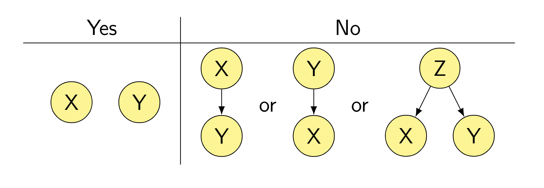
To address that question, we'll go to an example. Let and be two binary variables. Pearl asks: "Are and independent?" If yes, then there's no path between the two. If no, then there may be a path from to , or from to , or from a third variable to both and .
In either case, we're not going to infer any temporal relationships.
To me, it feels like this is where the adage "correlation does not imply causation" comes from. Pearl really needs more variables in order to be able to infer temporal relationships from more rich combinatorial structures.
However, I claim that this Pearlian ontology in which you're handed this collection of variables has blinded us to the obvious next question, which is: is independent of ?
In the Pearlian world, and were our variables, and is just some random operation on those variables. In our world, instead is a variable on the same footing as and . The first thing I do with my variables and is that I take the product and then I forget the labels and .
So there's this question, "Is independent of ?". And if is independent of , we're actually going to be able to conclude that is before !
So not only is the finite factored set paradigm non-vacuous, and not only is it going to be able to keep up with Pearl and infer things Pearl can't, but it's going to be able to infer a temporal relationship from only two variables.
So let's go through the proof of that.
2e.
Let , and let , , and be the partitions (/questions):
- . (What is the first bit?)
- . (What is the second bit?)
- . (Do the bits match?)
Let , where and . If we'd gotten this orthogonality database from a probability distribution, then we would have more than just two rules, since we would observe more orthogonality and non-orthogonality than that. But temporal inference is monotonic with respect to adding more rules, so we can just work with the smallest set of rules we'll need for the proof.
The first rule says that is orthogonal to . The second rule says that is not orthogonal to itself, which is basically just saying that is non-deterministic; it's saying that both of the parts in are possible, that both are supported under the function . The indicates that we aren't making any conditions.
From this, we'll be able to prove that .
Proof. First, we'll show that that is weakly before . Let satisfy . Let be shorthand for , and likewise let and .
Since , we have that ; and since , we have that .
Since —that is, since can be computed from together with —. (Because a partition's history is the smallest set of factors needed to compute that partition.)
And since , this implies , so is weakly before .
To show the strict inequality, we'll assume for the purpose of contradiction that = .
Notice that can be computed from together with —that is, —and therefore (i.e., ). It follows that . But since is also disjoint from , this means that , a contradiction.
Thus , so , so , so .
When I'm doing temporal inference using finite factored sets, I largely have proofs that look like this. We collect some facts about emptiness or non-emptiness of various Boolean combinations of histories of variables, and we use these to conclude more facts about histories of variables being subsets of each other.
I have a more complicated example that uses conditional orthogonality, not just orthogonality; I'm not going to go over it here.
One interesting point I want to make here is that we're doing temporal inference—we're inferring that is before —but I claim that we're also doing conceptual inference.
Imagine that I had a bit, and it's either a 0 or a 1, and it's either blue or green. And these two facts are primitive and independently generated. And I also have this other concept that's like, "Is it grue or bleen?", which is the of blue/green and 0/1.
There's a sense in which we're inferring is before , and in that case, we can infer that blueness is before grueness. And that's pointing at the fact that blueness is more primitive, and grueness is a derived property.
In our proof, and can be thought of as these primitive properties, and is a derived property that we're getting from them. So we're not just inferring time; we're inferring facts about what are good, natural concepts. And I think that there's some hope that this ontology can do for the statement "you can't really distinguish between blue and grue" what Pearl can do to the statement "correlation does not imply causation".
2b.
The future work I'm most excited by with finite factored sets falls into three rough categories: inference (which involves more computational questions), infinity (more mathematical), and embedded agency (more philosophical).
Research topics related to inference:
- Decidability of Temporal Inference
- Efficient Temporal Inference
- Conceptual Inference
- Temporal Inference from Raw Data and Fewer Ontological Assumptions
- Temporal Inference with Deterministic Relationships
- Time without Orthogonality
- Conditioned Factored Sets
There are a lot of research directions suggested by questions like "How do we do efficient inference in this paradigm?". Some of the questions here come from the fact that we're making fewer assumptions than Pearl, and are in some sense more coming from the raw data.
Then I have the applications that are about extending factored sets to the infinite case:
- Extending Definitions to the Infinite Case
- The Fundamental Theorem of Finite-Dimensional Factored Sets
- Continuous Time
- New Lens on Physics [LW · GW]
Everything I've presented in this talk was under the assumption of finiteness. In some cases this wasn't necessary—but in a lot of cases it actually was, and I didn't draw attention to this.
I suspect that the fundamental theorem can be extended to finite-dimensional factored sets (i.e., factored sets where is finite), but it can not be extended to arbitrary-dimension factored sets.
And then, what I'm really excited about is applications to embedded agency:
- Embedded Observations
- Counterfactability
- Cartesian Frames [LW · GW] Successor
- Unraveling Causal Loops [LW · GW]
- Conditional Time
- Logical Causality from Logical Induction
- Orthogonality as Simplifying Assumptions for Decisions
- Conditional Orthogonality as Abstraction Desideratum
I focused on the temporal inference aspect of finite factored sets in this talk, because it's concrete and tangible to be able to say, "Ah, we can do Pearlian temporal inference, only we can sometimes infer more structure and we rely on fewer assumptions."
But really, a lot of the applications I'm excited about involve using factored sets to model situations, rather than inferring factored sets from data.
Anywhere that we currently model a situation using graphs with directed edges that represent information flow or causality, we might instead be able to use factored sets to model the situation; and this might allow our models to play more nicely with abstraction.
I want to build up the factored set ontology as an alternative to graphs when modeling agents interacting with things, or when modeling information flow. And I'm really excited about that direction.
95 comments
Comments sorted by top scores.
comment by paulfchristiano · 2021-05-24T18:56:56.608Z · LW(p) · GW(p)
Here is how I'm currently thinking about this framework and especially inference, in case it's helpful for other folks who have similar priors to mine (or in case something is still wrong).
A description of traditional causal models:
- A causal graph with N nodes can be viewed as a model with 2N variables, one for each node of the graph and a corresponding noise variable for each. Each real variable is a deterministic function of its corresponding noise variable + its parents in the causal graph.
- When we talk about causal inference, we often consider probabilities in "generic position": we ask what kind of graphs would give rise to the observed conditional independence relations (and no others) regardless of the probability distributions and functions.
In the factored sets framework:
- We still posit a bunch of independent noise variables, and our observations are still a deterministic functions of these noise variables.
- But we no longer make any structural assumption about an underlying graph---the deterministic functions can be arbitrary.
- It's easy to prove that for any deterministic function there is a unique "smallest" set of variables on which it potentially depends. We call this the history.
- Now we define "Y is after X" to mean that X depends on a strict subset of the variables on which Y depends.
- (For a traditional causal model, this is equivalent to the usual definition, since the history of a variable is the set of noise variables upstream of it.)
- We can ask the same kinds of questions we asked before: what properties are true about all models that can give rise to the observed conditional independence relations (and no others) regardless of the probability distribution on the noise variables. For example, we can ask whether "Y is after X" is true in all of these models.
Some other thoughts:
- We can enlarge Pearl's framework to allow deterministic nodes. If we do, both of these frameworks are compatible with the same set of distributions about the world (and can represent the same sets of distributions when we take the probabilities to be arbitrary, as long as we allow the deterministic nodes to be fixed).
- But this makes it hard to say much of anything in Pearl's framework. The basic problem is that for all you know Pearl's models now look like the factored sets models---there could be a bunch of independent random variables, and then everything we observe is a deterministic function of them. In fact this seems like a pretty natural view of the real world. In this case there are no causal relationships between anything we observe, and it just feels like many of Pearl's definitions aren't a good fit. (I initially thought the d-separation criterion still worked but Scott points out that it definitely doesn't.)
- I think the definition of history is the most natural way to recover something like causal structure in these models. I can't think of any other good options, and I don't currently see any major downsides or intuition-violations in this approach. And then as far as I can tell most everything else follows naturally from this key assumption (I haven't thought about alternative definitions of conditional orthogonality but it feels intuitively like there must be only one reasonable definition).
- It's not a priori clear to me whether or not the fundamental theorem would hold. But it clearly should if this notion of history/orthogonality is a good one. Given that it holds I'm inclined to accept this as a good generalization of Pearl's notion to models with determinism / with more events than noise variables. I'd expect to revise that position if someone turned up a case where the definitions felt wrong, or if someone was able to offer a similarly-compelling alternative.
- I'm not a big fan of the name "finite factored sets" because it feels to me like it doesn't emphasize the most important difference between these frameworks. Maybe my perspective on the terminology would shift if I thought about it more.
↑ comment by cousin_it · 2021-05-25T10:40:04.085Z · LW(p) · GW(p)
I think the definition of history is the most natural way to recover something like causal structure in these models.
I'm not sure how much it's about causality. Imagine there's a bunch of envelopes with numbers inside, and one of the following happens:
-
Alice peeks at three envelopes. Bob peeks at ten, which include Alice's three.
-
Alice peeks at three envelopes and tells the results to Bob, who then peeks at seven more.
-
Bob peeks at ten envelopes, then tells Alice the contents of three of them.
Under the FFS definition, Alice's knowledge in each case is "strictly before" Bob's. So it seems less of a causal relationship and more like "depends on fewer basic facts".
Replies from: paulfchristiano↑ comment by paulfchristiano · 2021-05-25T16:18:00.283Z · LW(p) · GW(p)
Agree it's not totally right to call this a causal relationship.
That said:
- The contents of 3 envelopes does seems causally upstream of the contents of 10 envelopes
- If Alice's perception is imperfect (in any possible world), then "what Alice perceived" is not identical to "the contents of 3 envelopes" and so is not strictly before "what Bob perceived" (unless there is some other relationship between them).
- If Alice's perception is perfect in every possible world, then there is no possible way to intervene on Alice's perception without intervening on the contents of the 3 envelopes. So it seems like a lot rests on whether you are restricting your attention to possible worlds.
- Even if Alice's perception is perfect (or if Bob is guaranteed to tell Alice the contents of the 3 envelopes) we can still imagine an intervention on Alice's perception, and in your stories it seems like that's what makes it feel like Alice's perception isn't upstream of Bob's perception. But it feels to me like this imagination ought to track subjective possibility, even if in fact it is probably logically necessary that Alice perceives correctly / Bob reports correctly / whatever.
So I do feel like there's a case to be made that it captures everything we should care about with respect to causality.
For example, it seems unlikely to me that decision theory should depend on what happens in obviously impossible worlds. If we want to depend on impossible worlds it seems like it will usually happen by introducing a more naive epistemic state from which those worlds are subjectively possible---in which case we can talk about the FFS definition with respect to that epistemic state.
(I have no idea if this perspective is endorsed by Scott or if it would stand up to scrutiny.)
Replies from: Scott Garrabrant, cousin_it↑ comment by Scott Garrabrant · 2021-05-25T16:27:37.078Z · LW(p) · GW(p)
I think I (at least locally) endorse this view, and I think it is also a good pointer to what seems to me to be the largest crux between the my theory of time and Pearl's theory of time.
↑ comment by cousin_it · 2021-05-26T09:14:19.403Z · LW(p) · GW(p)
I feel that interpreting "strictly before" as causality is making me more confused.
For example, here's a scenario with a randomly changed message. Bob peeks at ten regular envelopes and a special envelope that gives him a random boolean. Then Bob tells Alice the contents of either the first three envelopes or the second three, depending on the boolean. Now Alice's knowledge depends on six out of ten regular envelopes and the special one, so it's still "strictly before" Bob's knowledge. And since Alice's knowledge can be computed from Bob's knowledge but not vice versa, in FFS terms that means the "cause" can be (and in fact is) computed from the "effect", but not vice versa. My causal intuition is just blinking at all this.
Here's another scenario. Alice gets three regular envelopes and accurately reports their contents to Bob, and a special envelope that she keeps to herself. Then Bob peeks at seven more envelopes. Now Alice's knowledge isn't "before" Bob's, but if later Alice predictably forgets the contents of her special envelope, her knowledge becomes "before" Bob's. Even though the special envelope had no effect on the information Alice gave to Bob, didn't affect the causal arrow in any possible world. And if we insist that FFS=causality, then by forgetting the envelope, Alice travels back in time to become the cause of Bob's knowledge in the past. That's pretty exotic.
Replies from: Scott Garrabrant↑ comment by Scott Garrabrant · 2021-05-26T17:50:11.551Z · LW(p) · GW(p)
I partially agree, which is partially why I am saying time rather than causality.
I still feel like there is an ontological disagreement in that it feels like you are objecting to saying the physical thing that is Alice's knowledge is (not) before the physical thing that is Bob's knowledge.
In my ontology:
1) the information content of Alice's knowledge is before the information content of Bob's knowledge. (I am curios if this part is controversial.)
and then,
2) there is in some sense no more to say about the physical thing that is e.g. Alice's knowledge beyond the information content.
So, I am not just saying Alice is before Bob, I am also saying e.g. Alice is before Alice+Bob, and I can't disentangle these statements because Alice+Bob=Bob.
I am not sure what to say about the second example. I am somewhat rejecting the dynamics. "Alice travels back in time" is another way of saying that the high level FFS time disagrees with the standard physical time, which is true. The "high level" here is pointing to the fact that we are only looking at the part of Alice's brain that is about the envelopes, and thus talking about coarser variables than e.g. Alice's entire brain state in physical time. And if we are in the ontology where we are only looking at the information content, taking a high level version of a variable is the kind of thing that can change its temporal properties, since you get an entirely new variable.
I suspect most of the disagreement is in the sort of "variable nonrealism" of reducing the physical thing that is Alice's knowledge to its information content?
Replies from: cousin_it↑ comment by cousin_it · 2021-05-26T18:37:34.133Z · LW(p) · GW(p)
Not sure we disagree, maybe I'm just confused. In the post you show that if X is orthogonal to X XOR Y, then X is before Y, so you can "infer a temporal relationship" that Pearl can't. I'm trying to understand the meaning of the thing you're inferring - "X is before Y". In my example above, Bob tells Alice a lossy function of his knowledge, and Alice ends up with knowledge that is "before" Bob's. So in this case the "before" relationship doesn't agree with time, causality, or what can be computed from what. But then what conclusions can a scientist make from an inferred "before" relationship?
Replies from: Scott Garrabrant↑ comment by Scott Garrabrant · 2021-05-26T22:00:04.291Z · LW(p) · GW(p)
I don't have a great answer, which isn't a great sign.
I think the scientist can infer things like. "algorithms reasoning about the situation are more likely to know X but not Y than they are to know Y but not X, because reasonable processes for learning Y tend to learn learn enough information to determine X, but then forget some of that information." But why should I think of that as time?
I think the scientist can infer things like "If I were able to factor the world into variables, and draw a DAG (without determinism) that is consistent with the distribution with no spurious independencies (including in deterministic functions of the variables), and X and Y happen to be variables in that DAG, then there will be a path from X to Y."
The scientist can infer that if Z is orthogonal to Y, then Z is also orthogonal to X, where this is important because Z is orthogonal to Y can be thought of as saying that Z is useless for learning about Y. (and importantly a version of useless for learning that is closed under common refinement, so if you collect a bunch of different Z orthogonal to Y, you can safely combine them, and the combination will be orthogonal to Y.)
This doesn't seem to get at why we want to call it before. Hmm.
Maybe I should just list a bunch of reasons why it feels like time to me (in no particular order):
- It seems like it gets a very reasonable answer in the Game of Life example
- Prior to this theory, I thought that it made sense to think of time as a closure property on orthogonality, and this definition of time is exactly that closure property on orthogonality, where X is weakly before Y if whenever Z is orthogonal to Y, Z is also orthogonal to X. (where the definition of orthogonality is justified with the fundamental theorem.)
- If Y is a refinement of X, then Y cannot be strictly before X. (I notice that I don't have a thing to say about why this feels like time to me, and indeed it feels like it is in direct opposition to your "doesn't agree with what can be computed from what," but it does agree with the way I feel like I want to intuitively describe time in the stories told in the "Saving Time" post.) (I guess one thing I can say is that as an agent learns over time, we think of the agent as collecting information, so later=more information makes sense.)
- History looks a lot like a non-quantitative version of entropy, where instead of thinking of how much randomness goes into a variable, we think of which randomness goes into the variable. There are lemmas towards proving the semigraphoid axioms which look like theorems about entropy modified to replace sums/expectations with unions. Then, "after" exactly corresponds to "greater entropy" in this analogy.
- If I imagine X and Z being computed independently, and Y as being computed from X and Z, it will say that X is before Y, which feels right to me (and indeed this property is basically the definition. It seems like my time is maybe the unique thing that gets the right answer on this simple story and also treats variables with the same info content as the same.)
- We can convert a Pearlian DAG to a FFS, and under this conversion, d-seperation is sent to conditional orthogonality, and paths between nodes are sent to time. (on the questions Pearl knows how to ask. We also generalize the definition to all variables)
↑ comment by cousin_it · 2021-05-26T22:40:49.673Z · LW(p) · GW(p)
Thanks for the response! Part of my confusion went away, but some still remains.
In the game of life example, couldn't there be another factorization where a later step is "before" an earlier one? (Because the game is non-reversible and later steps contain less and less information.) And if we replace it with a reversible game, don't we run into the problem that the final state is just as good a factorization as the initial?
Replies from: Scott Garrabrant↑ comment by Scott Garrabrant · 2021-05-27T00:38:00.674Z · LW(p) · GW(p)
Yep, there is an obnoxious number of factorizations of a large game of life computation, and they all give different definitions of "before."
Replies from: cousin_it↑ comment by cousin_it · 2021-05-27T10:00:55.818Z · LW(p) · GW(p)
I think your argument about entropy might have the same problem. Since classical physics is reversible, if we build something like a heat engine in your model, all randomness will be already contained in the initial state. Total "entropy" will stay constant, instead of growing as it's supposed to, and the final state will be just as good a factorization as the initial. Usually in physics you get time (and I suspect also causality) by pointing to a low probability macrostate and saying "this is the start", but your model doesn't talk about macrostates yet, so I'm not sure how much it can capture time or causality.
That said, I like really like how your model talks only about information, without postulating any magical arrows. Maybe it has a natural way to recover macrostates, and from them, time?
Replies from: Scott Garrabrant↑ comment by Scott Garrabrant · 2021-05-27T16:43:08.629Z · LW(p) · GW(p)
Wait, I misunderstood, I was just thinking about the game of life combinatorially, and I think you were thinking about temporal inference from statistics. The reversible cellular automaton story is a lot nicer than you'd think.
if you take a general reversible cellular automaton (critters for concreteness), and have a distribution over computations in general position in which initial conditions cells are independent, the cells may not be independent at future time steps.
If all of the initial probabilities are 1/2, you will stay in the uniform distribution, but if the probabilities are in general position, things will change, and time 0 will be special because of the independence between cells.
There will be other events at later times that will be independent, but those later time events will just represent "what was the state at time 0."
For a concrete example consider the reversible cellular automaton that just has 2 cells, X and Y, and each time step it keeps X constant and replaces Y with X xor Y.
Replies from: cousin_it, Scott Garrabrant, Scott Garrabrant↑ comment by cousin_it · 2021-05-27T18:07:36.885Z · LW(p) · GW(p)
Wait, can you describe the temporal inference in more detail? Maybe that's where I'm confused. I'm imagining something like this:
-
Check which variables look uncorrelated
-
Assume they are orthogonal
-
From that orthogonality database, prove "before" relationships
Which runs into the problem that if you let a thermodynamical system run for a long time, it becomes a "soup" where nothing is obviously correlated to anything else. Basically the final state would say "hey, I contain a whole lot of orthogonal variables!" and that would stop you from proving any reasonable "before" relationships. What am I missing?
Replies from: Scott Garrabrant↑ comment by Scott Garrabrant · 2021-05-27T18:44:27.074Z · LW(p) · GW(p)
I think that you are pointing out that you might get a bunch of false positives in your step 1 after you let a thermodynamical system run for a long time, but they are are only approximate false positives.
Replies from: cousin_it↑ comment by Scott Garrabrant · 2021-05-27T16:51:24.151Z · LW(p) · GW(p)
I think my model has macro states. In game of life, if you take the entire grid at time t, that will have full history regardless of t. It is only when you look at the macro states (individual cells) that my time increases with game of life time.
↑ comment by Scott Garrabrant · 2021-05-27T16:49:10.163Z · LW(p) · GW(p)
As for entropy, here is a cute observation (with unclear connection to my framework): whenever you take two independent coin flips (with probabilities not 0,1, or 1/2), their xor will always be high entropy than either of the individual coin flips.
↑ comment by Scott Garrabrant · 2021-05-24T19:19:48.104Z · LW(p) · GW(p)
Thanks Paul, this seems really helpful.
As for the name I feel like "FFS" is a good name for the analog of "DAG", which also doesn't communicate that much of the intuition, but maybe doesn't make as much sense for name of the framework.
Replies from: Scott Garrabrant, paulfchristiano↑ comment by Scott Garrabrant · 2021-05-24T19:30:37.783Z · LW(p) · GW(p)
I was originally using the name Time Cube, but my internal PR center wouldn't let me follow through with that :)
Replies from: gwillen↑ comment by paulfchristiano · 2021-05-24T21:12:44.438Z · LW(p) · GW(p)
I think FFS makes sense as an analog of DAG, and it seems reasonable to think of the normal model as DAG time and this model as FFS time. I think the name made me a bit confused by calling attention to one particular diff between this model and Pearl (factored sets vs variables), whereas I actually feel like that diff was basically a red herring and it would have been fastest to understand if the presentation had gone in the opposite direction by demphasizing that diff (e.g. by presenting the framework with variables instead of factors).
That said, even the DAG/FFS analogy still feels a bit off to me (with the caveat that I may still not have a clear picture / don't have great aesthetic intuitions about the domain).
Factorization seems analogous to describing a world as a set of variables (and to the extent it's not analogous it seems like an aesthetic difference about whether to take the world or variables as fundamental, rather than a substantive difference in the formalism) rather than to the DAG that relates the variables.
The structural changes seem more like (i) replacing a DAG with a bipartite graph, (ii) allowing arrows to be deterministic (I don't know how typically this is done in causal models). And then those structural changes lead to generalizing the usual concepts about causality so that they remain meaningful in this setting.
All that said, I'm terrible at both naming things and presenting ideas, and so don't want to make much of a bid for changes in either department.
Replies from: Scott Garrabrant↑ comment by Scott Garrabrant · 2021-05-24T21:49:00.901Z · LW(p) · GW(p)
Makes sense. I think a bit of my naming and presentation was biased by being so surprised by the not on OEIS fact.
I think I disagree about the bipartite graph thing. I think it only feels more natural when comparing to Pearl. The talk frames everything in comparison to Pearl, but I think if you are not looking at Pearl, I think graphs don’t feel like the right representation here. Comparing to Pearl is obviously super important, and maybe the first introduction should just be about the path from Pearl to FFS, but once we are working within the FFS ontology, graphs feel not useful. One crux might be about how I am excited for directions that are not temporal inference from statistical data.
My guess is that if I were putting a lot of work into a very long introduction for e.g. the structure learning community, I might start the way you are emphasizing, but then eventually convert to throwing all the graphs away.
(The paper draft I have basically only ever mentions Pearl/graphs for motivation at the beginning and in the applications section.)
Replies from: paulfchristiano↑ comment by paulfchristiano · 2021-05-24T23:09:10.282Z · LW(p) · GW(p)
I agree that bipartite graphs are only a natural way of thinking about it if you are starting from Pearl. I'm not sure anything in the framework is really properly analogous to the DAG in a causal model.
Replies from: Koen.Holtman↑ comment by Koen.Holtman · 2021-05-25T12:39:44.598Z · LW(p) · GW(p)
My thoughts on naming this finite factored sets: I agree with Paul's observation that
| Factorization seems analogous to describing a world as a set of variables
By calling this 'finite factored sets', you are emphasizing the process of coming up with individual random variables, the variables that end up being the (names of the) nodes in a causal graph. With representing the entire observable 4D history of a world (like a computation starting from a single game of life board state), a factorisation splits such into a tuple of separate, more basic observables . where , etc. In the normal narrative that explains Pearl causal graphs, this splitting of the world into smaller observables is not emphasized. Also, the splitting does not necessarily need to be a bijection. It may loose descriptive information with respect to .
So I see the naming finite factored sets as a way to draw attention to this splitting step, it draws attention to the fact that if you split things differently, you may end up with very different causal graphs. This leaves open the question of course is if really want to name your framework in a way that draws attention to this part of the process. Definitely you spend a lot of time on creating an equivalent to the arrows between the nodes too.
comment by Scott Garrabrant · 2021-05-26T17:06:45.886Z · LW(p) · GW(p)
Now on OEIS: https://oeis.org/A338681
comment by Rohin Shah (rohinmshah) · 2021-09-06T21:36:21.475Z · LW(p) · GW(p)
Planned summary for the Alignment Newsletter. I'd be particularly keen for someone to check that I didn't screw up in the section "Orthogonality in Finite Factored Sets":
This newsletter is a combined summary + opinion for the [Finite Factored Sets sequence](https://www.alignmentforum.org/s/kxs3eeEti9ouwWFzr [? · GW]) by Scott Garrabrant. I (Rohin) have taken a lot more liberty than I usually do with the interpretation of the results; Scott may or may not agree with these interpretations.
## Motivation
One view on the importance of deep learning is that it allows you to automatically _learn_ the features that are relevant for some task of interest. Instead of having to handcraft features using domain knowledge, we simply point a neural net at an appropriate dataset, and it figures out the right features. Arguably this is the _majority_ of what makes up intelligent cognition; in humans it seems very analogous to [System 1](https://en.wikipedia.org/wiki/Thinking,_Fast_and_Slow), which we use for most decisions and actions. We are also able to infer causal relations between the resulting features.
Unfortunately, [existing models](https://en.wikipedia.org/wiki/The_Book_of_Why) of causal inference don’t model these learned features -- they instead assume that the features are already given to you. Finite Factored Sets (FFS) provide a theory which can talk directly about different possible ways to featurize the space of outcomes, and still allows you to perform causal inference. This sequence develops this underlying theory, and demonstrates a few examples of using finite factored sets to perform causal inference given only observational data.
Another application is to <@embedded agency@>(@Embedded Agents@): we would like to think of “agency” as a way to featurize the world into an “agent” feature and an “environment” feature, that together interact to determine the world. In <@Cartesian Frames@>, we worked with a function A × E → W, where pairs of (agent, environment) together determined the world. In the finite factored set regime, we’ll think of A and E as features, the space S = A × E as the set of possible feature vectors, and S → W as the mapping from feature vectors to actual world states.
## What is a finite factored set?
Generalizing this idea to apply more broadly, we will assume that there is a set of possible worlds Ω, a set S of arbitrary elements (which we will eventually interpret as feature vectors), and a function f : S → Ω that maps feature vectors to world states. Our goal is to have some notion of “features” of elements of S. Normally, when working with sets, we identify a feature value with the set of elements that have that value. For example, we can identify “red” as the set of all red objects, and in [some versions of mathematics](https://en.wikipedia.org/wiki/Set-theoretic_definition_of_natural_numbers#Frege_and_Russell), we define “2” to be the set of all sets that have exactly two elements. So, we define a feature to be a _partition_ of S into subsets, where each subset corresponds to one of the possible feature values. We can also interpret a feature as a _question_ about items in S, and the values as possible _answers_ to that question; I’ll be using that terminology going forward.
A finite factored set is then given by (S, B), where B is a set of **factors** (questions), such that if you choose a particular answer to every question, that uniquely determines an element in S (and vice versa). We’ll put aside the set of possible worlds Ω; for now we’re just going to focus on the theory of these (S, B) pairs.
Let’s look at a contrived example. Consider S = {chai, caesar salad, lasagna, lava cake, sprite, strawberry sorbet}. Here are some possible questions for this S:
- **FoodType**: Possible answers are Drink = {chai, sprite}, Dessert = {lava cake, strawberry sorbet}, Savory = {caesar salad, lasagna}
- **Temperature**: Possible answers are Hot = {chai, lava cake, lasagna} and Cold = {sprite, strawberry sorbet, caesar salad}.
- **StartingLetter**: Possible answers are “C” = {chai, caesar salad}, “L” = {lasagna, lava cake}, and “S” = {sprite, strawberry sorbet}.
- **NumberOfWords**: Possible answers are “1” = {chai, lasagna, sprite} and “2” = {caesar salad, lava cake, strawberry sorbet}.
Given these questions, we could factor S into {FoodType, Temperature}, or {StartingLetter, NumberOfWords}. We _cannot_ factor it into, say, {StartingLetter, Temperature}, because if we set StartingLetter = L and Temperature = Hot, that does not uniquely determine an element in S (it could be either lava cake or lasagna).
Which of the two factorizations should we use? We’re not going to delve too deeply into this question, but you could imagine that if you were interested in questions like “does this need to be put in a glass” you might be more interested in the {FoodType, Temperature} factorization.
Just to appreciate the castle of abstractions we’ve built, here’s the finite factored set F with the factorization {FoodType, Temperature}:
F = ({chai, caesar salad, lasagna, lava cake, sprite, strawberry sorbet}, {{{chai, sprite}, {lava cake, strawberry sorbet}, {caesar salad, lasagna}}, {{chai, lava cake, lasagna}, {sprite, strawberry sorbet, caesar salad}}})
To keep it all straight, just remember: a **factorization** B is a set of **questions** (factors, partitions) each of which is a set of **possible answers** (parts), each of which is a set of elements in S.
## A brief interlude
Some objections you might have about stuff we’ve talked about so far:
**Q.** Why do we bother with the set S -- couldn’t we just have the set of questions B, and then talk about answer vectors of the form (a1, a2, … aN)?
**A.** You could in theory do this, as there is a bijection between S and the Cartesian product of the sets in B. However, the problem with this framing is that it is hard to talk about other derived features. For example, the question “what is the value of B1+B2” has no easy description in this framing. When we instead directly work with S, the B1+B2 question is just another partition of S, just like B1 or B2 individually.
**Q.** Why does f map S to Ω? Doesn’t this mean that a feature vector uniquely determines a world state, whereas it’s usually the opposite in machine learning?
**A.** This is true, but here the idea is that the set of features together captures _all_ the information within the setting we are considering. You could think of feature vectors in deep learning as only capturing an important subset of all of the features (which we’d have to do in practice since we only have bounded computation), and those features are not enough to determine world states.
## Orthogonality in Finite Factored Sets
We’re eventually going to use finite factored sets similarly to Pearlian causal models: to infer which questions (random variables) are conditionally independent of each other. However, our analysis will apply to arbitrary questions, unlike Pearlian models, which can only talk about independence between the predefined variables from which the causal model is built.
Just like Pearl, we will talk about _conditioning on evidence_: given evidence e, a subset of S, we can “observe” that we are within e. In the formal setup, this looks like erasing all elements that are not in e from all questions, answers, factors, etc.
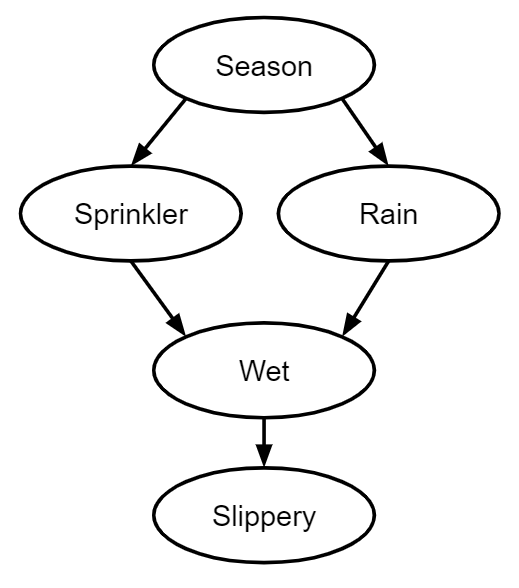
_Unlike_ Pearl, we’re going to assume that all of our factors are _independent_ from each other. In Pearlian causal models, the random variables are typically not independent from each other. For example, you might have a model with two binary variables, e.g. “Variable Rain causes Variable Wet Sidewalk”; these are obviously not independent. An analogous finite factored set would have _three_ factors: “did it rain?”, “if it rained did the sidewalk get wet?” and “if it didn’t rain did the sidewalk get wet?” This way all three factors can be independent of each other. We will still be able to ask whether Wet Sidewalk is independent of Rain, since Wet Sidewalk is just another question about the set S -- it just isn’t one of the underlying factors any more.
The point of this independence is to allow us to reason about _counterfactuals_: it should be possible to say “imagine the element s, except with underlying factor b2 changed to have value v”. As a result, our definitions will include clauses that say “and make sure we can still take counterfactuals”. For example, let’s talk about the “history” of a question X, which for now you can think of as the “factors relevant to X”. The _history_ of X given e is the smallest set of factors such that:
1) if you know the answers to these factors, then you can infer the answer to X, and
2) any factors that are _not_ in the history are independent of X. As suggested above, we can think of this as being about counterfactuals -- we’re saying that for any such factor, we can counterfactually change its answer, and this will remain consistent with the evidence e.
(A technicality on the second point: we’ll never be able to counterfactually change a factor to a value that is never found in the evidence; this is fine and doesn’t prevent things from being independent.)
Time for an example! Consider the set S = {000, 001, 010, 011, 100, 101, 110, 111}, and the factorization {X, Y, Z}, where X is the question “what is the first bit”, Y is the question “what is the second bit”, and Z is the question “what is the third bit”. Consider the question Q = “when interpreted as a binary number, is the number >= 2?” In this case, the history of Q given no evidence is {X, Y}, because you can determine the answer to Q with the combination of X and Y. (You can still counterfact on anything, since there is no evidence to be inconsistent with.)
Let’s consider an example with evidence. Suppose we observe that all the bits are equal, that is, e = {000, 111}. Now, what is the history of X? If there weren’t any evidence, the history would just be {X}; you only need to know X in order to determine the value of X. However, suppose we learned that X = 0, implying that our element is 000. We can’t counterfact on Y or Z, since that would produce 010 or 001, both of which are inconsistent with the evidence. So given this evidence, the history of X is actually {X, Y, Z}, i.e. the entire set of factors! If we’d only observed that the first two bits were equal, so e = {000, 001, 110, 111}, then we _could_ counterfact on Z, and the history of X would be {X, Y}.
(Should you want more examples, here are two [relevant](https://www.alignmentforum.org/posts/qGjCt4Xq83MBaygPx/a-simple-example-of-conditional-orthogonality-in-finite [AF · GW]) [posts](https://www.alignmentforum.org/posts/GFGNwCwkffBevyXR2/a-second-example-of-conditional-orthogonality-in-finite).)
Given this notion of “history”, it is easy to define orthogonality: X is orthogonal to Y given evidence e if the history of X given e has no overlap with the history of Y given e. Intuitively, this means that the factors relevant to X are completely separate from those relevant to Y, and so there cannot be any entanglement between X and Y. For a _question_ Z, we say that X is orthogonal to Y given Z if we have that X is orthogonal to Y given z, for every possible answer z in Z.
Now that we have defined orthogonality, we can state the _Fundamental Theorem of Finite Factored Sets_. Given some questions X, Y and Z about a finite factored set F, X is orthogonal to Y given Z if and only if in every probability distribution on F, X is conditionally independent of Y given Z, that is, P(X, Y | Z) = P(X | Z) * P(Y | Z).
(I haven’t told you how you put a probability distribution on F. It’s exactly what you would think -- you assign a probability to every possible answer in every factor, and then the probability of an individual element is defined to be the product of the probabilities of its answers across all the factors.)
(I also haven’t given you any intuition about why this theorem holds. Unfortunately I don’t have great intuition for this; the proof has multiple non-trivial steps each of which I locally understand and have intuition for... but globally it’s just a sequence of non-trivial steps to me. Here’s an attempt, which isn’t very good: we specifically defined orthogonality to capture *all* the relevant information for a question, in particular by having that second condition requiring that we be able to counterfact on other factors, and so it intuitively makes sense that if the relevant information doesn’t overlap then there can’t be a way for the probability distribution to have interactions between the variables.)
The fundamental theorem is in some sense a _justification_ for calling the property “orthogonality” -- if we determine just by studying the structure of the finite factored set that X is orthogonal to Y given Z, then we know that this implies conditional independence in the “true” probability distribution, whatever it ends up being. Pearlian models have a similar theorem, where the graphical property of d-separation implies conditional independence.
## Foundations of causality and time
You might be wondering why we have been calling the minimal set of relevant factors “history”. The core philosophical idea is that, if you have the right factorization, then “time” or “causality” can be thought of as flowing in the direction of larger histories. Specifically, we say that X is “before” Y if the history of X is a subset of the history of Y. (We then call it “history” because every factor in the history of X will be “before” X by this definition.)
One intuition pump for this is that in physics, if an event A causes an event B, then the past light cone of A is a subset of the past light cone of B, and A happens before B in every possible reference frame.
But perhaps the best argument for thinking of this as causality is that we can actually use this notion of “time” or “causality” to perform causal inference. Before I talk about that, let’s see what this looks like in Pearlian models.
Strictly speaking, in Pearlian models, the edges do not _have_ to correspond to causality: formally they only represent conditional independence assumptions on a probability distribution. However, consider the following Cool Fact: for some Pearlian models, if you have observational data that is generated from that model, you can recover the exact graphical structure of the generating model just by looking at the observational data. In this case, you really are inferring cause-and-effect relationships from observational data! (In the general case where the data is generated by an arbitrary model, you can recover a lot of the structure of the model, but be uncertain about the direction of some of the edges, so you are still doing _some_ causal inference from observational data.)
We will do something similar: we’ll use our notion of “before” to perform causal inference given observational data.
## Temporal inference: the three dependent bits
You are given statistical (i.e. observational) data for three bits: X, Y and Z. You quickly notice that it is always the case that Z = X xor Y (which implies that X = Y xor Z, and Y = Z xor X). Clearly, there are only two independent bits here, and the other bit is derived as the xor of the two independent bits. From the raw statistical data, can you tell which bits are the independent ones, and which one is the derived one, thus inferring which one was _caused_ by the other two? It turns out that you can!
Specifically, you want to look for which two bits are _orthogonal_ to each other, that is, you want to check whether we approximately have P(X, Y) = P(X) P(Y) (and similarly for other possible pairings). In the world where two of the bits were generated by a biased coin, you will find exactly one pair that is orthogonal in this way. (The case where the bits are generated by a fair coin is a special case; the argument won’t work there, but it’s in some sense “accidental” and happens because the probability of 0.5 is very special.)
Let’s suppose that the orthogonal pair was (X, Z). In this case, we can _prove_ that in _every_ finite factored set that models this situation, X and Z come “before” Y, i.e. their histories are strict subsets of Y’s history. Thus, we’ve inferred causality using only observational data! (And unlike with Pearlian models, we did this in a case where one “variable” was a deterministic function of two other “variables”, which is a type of situation that Pearlian models struggle to handle.)
## Future work
Remember that motivation section, a couple thousand words ago? We talked about how we can do causal inference with learned featurizations, and apply it to embedded agency. Well, we actually haven’t done that yet, beyond a few examples of causal inference (as in the example above). There is a lot of future work to be done in applying it to the case that motivated it in the first place. The author wrote up potential future work [here](https://www.alignmentforum.org/s/kxs3eeEti9ouwWFzr/p/yGFiw23pJ32obgLbw [? · GW]), which has categories for both causal inference and embedded agency, and also adds a third one: generalizing the theory to infinite sets. If you are interested in this framework, there are many avenues for pushing it forward.
comment by alkjash · 2021-07-07T20:15:13.057Z · LW(p) · GW(p)
Are there any interesting pure combinatorics problems about finite factored sets that you're interested in?
Replies from: Scott Garrabrant↑ comment by Scott Garrabrant · 2021-07-07T22:02:44.768Z · LW(p) · GW(p)
- Given a finite set of cardinality , find a computable upper bound on the largest finite factored set model that is combinatorially different from all smaller finite factored set models. (We say that two FFS models are combinatorially different if they say the same thing about the emptiness of all boolean combinations of histories and conditional histories of partitions of .) (Such an upper bound must exist because there are only finitely many combinatorially distinct FFS models, but a computable upper bound, would tell us that temporal inference is computable.)
- Prove the fundamental theorem for finite dimensional factored sets. (Seems likely combinatorial-ish, but I am not sure.)
- Figure out how to write a program to do efficient temporal inference on small examples. (I suspect this requires a bunch of combinatorial insights. By default this is very intractable, but we might be able to use math to make it easier.)
- Axiomatize complete consistent orthogonality databases (consistent means consistent with some model, complete means has an opinion on every possible conditional orthogonality) (To start, is it the case that compositional semigraphoid axioms already work?)
If by "pure" you mean "not related to history/orthogonality/time," then no, the structure is simple, and I don't have much to ask about it.
Replies from: alkjash↑ comment by alkjash · 2021-07-07T23:39:45.088Z · LW(p) · GW(p)
Right, the structure is quite simple. The only thing that came to mind about finite factored sets as combinatorial objects was studying the L-function of the number of them, which surely has some nice Euler product. Maybe you can write it as a product of standard zeta functions or something?
comment by habryka (habryka4) · 2023-01-07T00:27:01.614Z · LW(p) · GW(p)
I've thought a good amount about Finite Factored Sets in the past year or two, but I do sure keep going back to thinking about the world primarily in the form of Pearlian causal influence diagrams, and I am not really sure why.
I do think this one line by Scott at the top gave me at least one pointer towards what was happening:
but I'm trained as a combinatorialist, so I'm giving a combinatorics talk upfront.
In the space of mathematical affinities, combinatorics is among the branches of math I feel most averse to, and I think that explains a good part of the problem I have with the current Finite Factored Sets explanation. I quite liked Paul's top comment, which characterized FFS as more of a generalization of Pearlian causality in a way that gave me a bit more of an in, but I do wish this sequence and talk would generally do that more, and maybe phrase things in a way that my graph-shaped, linear-algebra-shaped brain can more easily understand.
Replies from: Scott Garrabrant↑ comment by Scott Garrabrant · 2023-01-07T21:52:56.694Z · LW(p) · GW(p)
This [? · GW] underrated post is pretty good at explaining how to translate between FFSs and DAGs.
comment by Gurkenglas · 2021-06-03T09:02:21.391Z · LW(p) · GW(p)
Let's try category theory.
A partition is a family of sets called parts. A partition morphism X->X' has a function from each part of X to some part of X'. It witnesses that X is finer than X'¹.
The underlying set of a partition is its disjoint union. Call the discrete partition of S DS. The functions S->⊔X correspond to the partition morphisms DS->X. Call the trivial partition of S TS. The functions ⊔X->S correspond to the partition morphisms X->TS. In terser notation, we have D ⊣ ⊔ ⊣ T.
A factorization is a family of partitions called factors. A factorization morphism B->B' has a partition morphism to each factor of B' from some factor of B.²
The underlying partition of a factorization is its common refinement. Call the trivial factorization of X FX.³ The partition morphisms X->∨B correspond to the factorization morphisms FX->B: We have F ⊣ ∨. The absence of "discrete factorizations" as a right adjoint to ∨ is where histories come from.
A history of ∨B->X is a nice⁴ B->H with a ∨H->X. The history of ∨B->X is its terminal history. Note that this also attempts to coarsen each factor. ∨B->X being weakly after ∨B->X' is witnessed by a nice ∨H->X' or equivalently H->H'. ∨B->X and ∨B->X' are orthogonal iff the pushout of B->H and B->H' is the empty factorization.
Translating "2b. Conditional Orthogonality" is taking a while (I think it's something with pushouts) so let's post this now. I'm also planning to generalize "family" to "diagram". Everyone's allowed to ask stupid questions, including basic category theory.
¹: Which includes that X might rule out some worlds.
²: Trying to avert the analogy break cost me ~60% of the time behind this comment.
³: F for free, as in the left adjoint, and as in factorization.
⁴: Nice means that everything in sight commutes.
↑ comment by Gurkenglas · 2021-06-03T20:44:11.192Z · LW(p) · GW(p)
Let 1 be the category with one object • and one morphism. Let Δx be the constant functor to x.
A set is a family of • called elements. A set morphism S->S' has a 1-morphism between each element of S and some element of S'. The 1-morphisms •->Δ•S correspond to the set morphisms Δ∅•->S. The 1-morphisms Δ•S->• correspond to the set morphisms S->Δ1•. We have Δ∅ ⊣ Δ• ⊣ Δ1.
Let 0 the empty category. • is the empty family. A 1-morphism has nothing to prove. There's no forgetful functor 1->0 so the buck stops here.
↑ comment by Gurkenglas · 2021-06-04T16:27:12.205Z · LW(p) · GW(p)
Call the index set of X IX. Call the partition into empty parts indexed by S 0S. We have 0 ⊣ I ⊣ D ⊣ ⊔ ⊣ T.
None of the our three adjunction strings can be extended further. Let's apply the construction that gave us histories at the other 5 ends. Niceness is implicit.
- The right construction of TS->X is the terminal S->S' with a TS'->X: The image of ⊔(TS->X).
- The left construction of X->0S is the initial S'->S with a X->0S': The image of I(X->0S).
- The left construction of B->FX is the initial X'->X with a B->FX': The image of ∨(B->FX).
- The right construction of Δ1•->S is the terminal •->• with a Δ1•->S: The image of Δ•(Δ1•->S).
- The left construction of S->Δ∅• is absurd, but can still be written as the image of Δ•(S->Δ∅•).
- The history of ∨B->X is the terminal B->B' with a ∨B'->X: Breaks the pattern! F(∨B->X) does not have the information to determine the history.
In fact, ⊔T, I0, ∨F, Δ•Δ1 and Δ•Δ∅ are all identity, only F∨ isn't.
comment by michaelcohen (cocoa) · 2021-05-24T12:53:21.510Z · LW(p) · GW(p)
I was thinking of some terminology that might make it easier to thinking about factoring and histories and whatnot.
A partition can be thought of as a (multiple-choice) question. Like for a set of words, you could have the partition corresponding to the question "Which letter does the word start with?" and then the partition groups together elements with the same answer.
Then a factoring is set of questions, where the set of answers will uniquely identify an element. The word that comes to mind for me is "signature", where an element's signature is the set of answers to the given set of questions.
For the history of a partition X, X can be thought of as a question, and the history is the subset of questions in the factoring that you need the answers to in order to determine the answer to question X.
And then two questions X and Y are orthogonal if there aren't any questions in the factoring that you need the answer to both for answering X and for answering Y.
Replies from: Scott Garrabrant↑ comment by Scott Garrabrant · 2021-05-24T15:49:35.109Z · LW(p) · GW(p)
Yep, this all seems like a good way of thinking about it.
comment by JenniferRM · 2021-05-24T04:31:21.390Z · LW(p) · GW(p)
I have read most of the article, but not yet carefully combed the math or watched the video.
The OEIS gap seems suggestive of "being on the track of something novel (and thus maybe novel and good)".
Reading this, some things clicked for me as "possibly related and worth looking at" that I hadn't really noticed before.
Specifically, I was reminded of how "TF * IDF" is this old pragmatic "it works in practice" mathematical kludge for information retrieval that just... gets the job done better "with" than "without" nearly all of the time? People have ideas why it works, but then they start debating the tiny details and I don't think there's ever been a final perfectly coherent answer?
One framing idea might be "everything that works is actually Bayesian under the hood" and there's a small literature on "how to understand TF * IDF in Bayesian terms" that was reviewed by Robertson in 2004.
Long story, short: Event Spaces! (And 80/20 power laws?)
"The event space of topics, and of documents in topics, and of words in documents in topics" versus "the event space of queries, and of words in queries" and so on... If you make some plausible assumptions about the cartesian product (ahem!) of these event spaces, and how they relate to each other... maybe TF * IDF falls out as a fast/efficient approximation of a pragmatic approximation to "bayesian information retrieval"?
Something I noticed from reading about Finite Factored Sets was that I never really think much about what Pearl's causal graphs would look like if imagined in terms of bayesian event spaces... which I had never noticed as a gap in my thinking before today.
comment by ESRogs · 2021-05-24T03:08:22.177Z · LW(p) · GW(p)
Let , where and
[...] The second rule says that is orthogonal to itself
Should that be "is not orthogonal to itself"? I thought the meant non-orthogonal, so would think means that is not orthogonal to itself.
(The transcript accurately reflects what was said in the talk, but I'm asking whether Scott misspoke.)
↑ comment by Scott Garrabrant · 2021-05-24T03:25:07.689Z · LW(p) · GW(p)
Yeah, you are right. I will change it. Thanks.
comment by cousin_it · 2021-05-24T00:43:42.608Z · LW(p) · GW(p)
And if X is independent of X XOR Y, we’re actually going to be able to conclude that X is before Y!
It's interesting to translate that to the language of probabilities. For example, your condition holds for any X,Y (possibly dependent) such that P(X)=P(Y)=1/2, but it doesn't make sense to say that X is before Y in every such pair. For a real world example, take X = "person has above median height" and Y = "person has above median age".
Replies from: Scott Garrabrant↑ comment by Scott Garrabrant · 2021-05-24T01:06:16.273Z · LW(p) · GW(p)
So you should probably not work with probabilities equal to 1/2 in this framework, unless you are doing so for a specific reason. Just like in Pearlian causality, we are mostly talking about probabilities in general position. I have some ideas about how to deal with probability 1/2 (Have a FFS, together with a group of symmetry constraints, which could swap factors, or swap parts within a factor), but that is outside of the scope of what I am doing here.
To give more detail, the uniform distribution on four elements does not satisfy the compositional semigraphoid axioms, since if we take X, Y, Z to be the three partitions into two parts of size two, X is independent with Y and X is independent with Z, but X is not independent with the common refinement of Y and Z. Thus, if we take the orthogonality database generated by this probability distribution, you will find that it is not satisfied by any models.
Replies from: Scott Garrabrant, eigil-rischel↑ comment by Scott Garrabrant · 2021-05-24T01:13:07.524Z · LW(p) · GW(p)
The swapping within a factor allows for considering rational probabilities to be in general position, and the swapping factors allows IID samples to be considered in general position. I think this is an awesome research direction to go in, but it will make the story more complicated, since will not be able to depend on the fundamental theorem, since we are allowing for a new source of independence that is not orthogonality. (I want to keep calling the independence that comes from disjoint factors orthogonality, and not use "orthogonality" to describe the new independences that come from the principle of indifference.)
Replies from: cousin_it↑ comment by cousin_it · 2021-05-24T01:30:36.954Z · LW(p) · GW(p)
Yeah, that's what I thought, the method works as long as certain "conspiracies" among probabilities don't happen. (1/2 is not the only problem case, it's easy to find others, but you're right that they have measure zero.)
But there's still something I don't understand. In the general position, if X is before Y, it's not always true that X is independent of X XOR Y. For example, if X = "person has a car on Monday" and Y = "person has a car on Tuesday", and it's more likely that a car-less person gets a car than the other way round, the independence doesn't hold. It requires a conspiracy too. What's the intuitive difference between "ok" and "not ok" conspiracies?
Replies from: Scott Garrabrant↑ comment by Scott Garrabrant · 2021-05-24T01:46:48.626Z · LW(p) · GW(p)
I don't understand what conspiracy is required here.
X being orthogonal to X XOR Y implies X is before Y, we don't get the converse.
Replies from: cousin_it, acgt↑ comment by cousin_it · 2021-05-24T11:57:11.539Z · LW(p) · GW(p)
Well, imagine we have three boolean random variables. In "general position" there are no independence relations between them, so we can't say much. Constrain them so two of the variables are independent, that's a bit less "general", and we still can't say much. Constrain some more so the xor of all three variables is always 1, that's even less "general", now we can use your method to figure out that the third variable is downstream of the first two. Constrain some more so that some of the probabilities are 1/2, and the method stops working. What I'd like to understand is the intuition, which real world cases have the particular "general position" where the method works.
Replies from: Scott Garrabrant, acgt↑ comment by Scott Garrabrant · 2021-05-24T15:38:37.019Z · LW(p) · GW(p)
Ok, makes sense. I think you are just pointing out that when I am saying "general position," that is relative to a given structure, like FFS or DAG or symmetric FFS.
If you have a probability distribution, it might be well modeled by a DAG, or a weaker condition is that it is well modeled by a FFS, or an even weaker condition is that it is well modeled by a SFFS (symmetric finite factored set).
We have a version of the fundamental theorem for DAGs and d-seperation, we have a version of the fundamental theorem for FFS and conditional orthogonality, and we might get a version of the fundamental theorem for SFFS and whatever corresponds to conditional independence in that world.
However, I claim that even if we can extend to a fundamental theorem for SFFS, I still want to think of the independences in a SFFS as having different sources. There are the independences coming from orthogonality, and there are there the independences coming from symmetry (or symmetry together with orthogonality.
In this world, orthogonality won't be as inferable because it will only be a subset of independence, but it will still be an important concept. This is similar to what I think will happen when we go to the infinite dimensional factored sets case.
Replies from: cousin_it↑ comment by cousin_it · 2021-05-24T16:03:37.718Z · LW(p) · GW(p)
Can you give some more examples to motivate your method? Like the smoking/tar/cancer example for Pearl's causality, or Newcomb's problem and counterfactual mugging for UDT.
Replies from: Scott Garrabrant↑ comment by Scott Garrabrant · 2021-05-24T16:35:24.657Z · LW(p) · GW(p)
Hmm, first I want to point out that the talk here sort of has natural boundaries around inference, but I also want to work in a larger frame that uses FFS for stuff other than inference.
If I focus on the inference question, one of the natural questions that I answer is where I talk about grue/bleen in the talk.
I think for inference, it makes the most sense to think about FFS relative to Pearl. We have this problem with looking at smoking/tar/cancer, which is what if we carved into variables the wrong way. What if instead of tar/cancer, we had a variable for "How much bad stuff is in your body?" and "What is the ratio of tar to cancer?" The point is that our choice of variables both matters for the Pearlian framework, and is not empirically observable. I am trying to do all the good stuff in Pearl without the dependence on the variables
Indeed, I think the largest crux between FFS and Pearl is something about variable realism. To FFS, there is no realism to a variable beyond its information content, so it doesn't make sense to have two variables X, X' with the same information, but different temporal properties. Pearl's ontology, on the other hand, has these graphs with variables and edges that say "who listens to whom," which sets us up to be able to have e.g. a copy function from X to X', and an arrow from X to Y, which makes us want to say X is before Y, but X' is not.
For the more general uses of FFS, which are not about inference, my answer is something like "the same kind of stuff as Cartesian frames." e.g. specifying embedded observations. (A partition observes a subset relative to a high level world model if and . Notice the first condition is violated by transparent Newcomb, and the second condition is violated by counterfactual mugging. (The symbols here should be read as combinatorial properties, there are no probabilities involved.))
I want to be able to tell the stories like in the Saving Time [LW · GW] post, where there are abstract versions of things that are temporally related.
Replies from: Scott Garrabrant, cousin_it↑ comment by Scott Garrabrant · 2021-05-24T17:47:50.483Z · LW(p) · GW(p)
Here is a more concrete example of me using FFS the way I intend them to be used outside of the inference problem. (This is one specific application, but maybe it shows how I intend the concepts to be manipulated).
I can give an example of embedded observation maybe, but it will have to come after a more formal definition of observation (This is observation of a variable, rather than the observation of an event above):
Definition: Given a FFS , and , , , which are partitions of , where , we say observes relative to W if:
1) ,
2) can be expressed in the form , and
3) .
(This should all be interpreted combinatorially, not probabilistically.)
The intuition of what is going on here is that to observe an event, you are being promised that you 1) do not change whether the event holds, and 3) do not change anything that matters in the case where that event does not hold. Then, to observe a variable, you can basically 2) split yourself up into different fragments of your policy, where each policy fragment observes a different value of that variable. (This whole thing is very updateless.)
Example 1: (non-observation)
An agent does not observe a coinflip , and chooses to raise either his left or right hand. Our FFS is given by , and . (I am abusing notation here slightly by conflating with the partition you get on by projecting onto the coordinate.) Then W is the discrete partition on .
In this example, we do not have observation. Proof: A only has two parts, so if we express A as a common refinement of 2 partitions, at least one of these two partitions must be equal to A. However, A is not orthogonal to W given H and A is not orthogonal to W given T. (). Thus we must violate condition 3.
Example 2: (observation)
An agent does observe a coinflip , and chooses to raise either his left or right hand. We can think of as actually choosing a policy that is a function from to , where the two character string in the parts in are the result of H followed by the result of T.
Our FFS is given by , and , where represents what the agent would do seeing heads, and represents what the agent word do given seeing tails. . We also have a partition representing what the agent actually does , where and are each four element sets in the obvious way. We will then say , so W does not get to see what would have done, it only gets to see the coin flip and what actually did.
Now I will prove that observes relative to in this example. First, , and , so we get the first condition, . We will break up A in the obvious way set up in the problem for condition 2, so it suffices now to show that , (and it will follow symmetrically that .)
Im not going to go through the details, but , while , which are disjoint. The important thing here is that doesn't care about in worlds in which holds.
Discussion:
So largely I am sharing this to give an example for how you can manipulate FFS combinatorially, and how you can use this to say things that you might otherwise want to say using graphs, Granted, you could also say the above things using graphs, but now you can say more things, because you are not restricted to the nodes you choose, you can ask the same combinatorial question about any of the other partitions, The benefit is largely about not being dependent on our choice of variables.
It is interesting to try to translate this definition of observation to transparent Newcomb or counterfactual mugging, and see how some of the orthogonalities are violated, and thus it does not count as an observation.
↑ comment by cousin_it · 2021-05-24T16:50:24.924Z · LW(p) · GW(p)
Replies from: Scott Garrabrant↑ comment by Scott Garrabrant · 2021-05-24T17:45:00.595Z · LW(p) · GW(p)
I'll try. My way of thinking doesn't use the examples, so I have to generate them for communication.
I can give an example of embedded observation maybe, but it will have to come after a more formal definition of observation (This is observation of a variable, rather than the observation of an event above):
Definition: Given a FFS , and , , , which are partitions of , where , we say observes relative to W if:
1) ,
2) can be expressed in the form , and
3) .
(This should all be interpreted combinatorially, not probabilistically.)
The intuition of what is going on here is that to observe an event, you are being promised that you 1) do not change whether the event holds, and 3) do not change anything that matters in the case where that event does not hold. Then, to observe a variable, you can basically 2) split yourself up into different fragments of your policy, where each policy fragment observes a different value of that variable. (This whole thing is very updateless.)
Example 1 (non-observation)
An agent does not observe a coinflip , and chooses to raise either his left or right hand. Our FFS is given by , and . (I am abusing notation here slightly by conflating with the partition you get on by projecting onto the coordinate.) Then W is the discrete partition on .
In this example, we do not have observation. Proof: A only has two parts, so if we express A as a common refinement of 2 partitions, at least one of these two partitions must be equal to A. However, A is not orthogonal to W given H and A is not orthogonal to W given T. (). Thus we must violate condition 3.
Example 2: (observation)
An agent does observe a coinflip , and chooses to raise either his left or right hand. We can think of as actually choosing a policy that is a function from to , where the two character string in the parts in are the result of H followed by the result of T.
Our FFS is given by , and , where represents what the agent would do seeing heads, and represents what the agent word do given seeing tails. . We also have a partition representing what the agent actually does , where and are each four element sets in the obvious way. We will then say , so W does not get to see what would have done, it only gets to see the coin flip and what actually did.
Now I will prove that observes relative to in this example. First, , and , so we get the first condition, . We will break up A in the obvious way set up in the problem for condition 2, so it suffices now to show that , (and it will follow symmetrically that .)
Im not going to go through the details, but , while , which are disjoint. The important thing here is that doesn't care about in worlds in which holds.
Discussion:
So largely I am sharing this to give an example for how you can manipulate FFS combinatorially, and how you can use this to say things that you might otherwise want to say using graphs, Granted, you could also say the above things using graphs, but now you can say more things, because you are not restricted to the nodes you choose, you can ask the same combinatorial question about any of the other partitions, The benefit is largely about not being dependent on our choice of variables.
It is interesting to try to translate this definition of observation to transparent Newcomb or counterfactual mugging, and see how some of the orthogonalities are violated, and thus it does not count as an observation.
↑ comment by acgt · 2021-05-24T12:33:46.864Z · LW(p) · GW(p)
I’m confused what necessary work the Factorisation is doing in these temporal examples - in your example A and B are independent and C is related to both - the only assignment of “upstream/downstream” relations that makes sense is that C is downstream of both.
Is the idea that factorisation is what carves your massive set of possible worlds up into these variables in the first place? Feel like I’m in a weird position where the math makes sense but I’m missing the motivational intuition for why we want to switch to this framework in the first place
Replies from: Scott Garrabrant↑ comment by Scott Garrabrant · 2021-05-24T16:11:48.089Z · LW(p) · GW(p)
I are note sure what you are asking (indeed I am not sure if you are responding to me or cousin_it.)
One thing that I think is going on is that I use "factorization" in two places. Once when I say Pearl is using factorization data, and once where I say we are inferring a FFS. I think this is a coincidence. "Factorization" is just a really general and useful concept.
So the carving into A and B and C is a factorization of the world into variables, but it is not the kind of factorization that shows up in the FFS, because disjoint factors should be independent in the FFS.
As for why to switch to this framework, the main reason (to me) is that it has many of the advantages of Pearl with also being able to talk about some variables being coarse abstract versions of other variables. This is largely because I am interested in embedded agency applications.
Another reason is that we can't tell a compelling story about where the variables came from in the Pearlian story. Another reason is that sometimes we can infer time where Pearl cannot.
↑ comment by acgt · 2021-05-24T11:31:06.515Z · LW(p) · GW(p)
What would such a distribution look like? The version where X XOR Y is independent of both X and Y makes sense but I’m struggling to envisage a case where it’s independent of only 1 variable.
Replies from: Scott Garrabrant↑ comment by Scott Garrabrant · 2021-05-24T15:25:15.287Z · LW(p) · GW(p)
It looks like X and V are independent binary variables with different probabilities in general position, and Y is defined to be X XOR V. (and thus V=X XOR Y).
↑ comment by Eigil Rischel (eigil-rischel) · 2021-06-03T14:58:39.773Z · LW(p) · GW(p)
Thanks (to both of you), this was confusing for me as well.
comment by Jimdrix_Hendri · 2021-05-27T13:48:25.760Z · LW(p) · GW(p)
Cool topic!
Here are some critiques on part 1 of your presentation: Short Combinatorial Talk
1 Colour coding slides by content is a nifty idea. I hadn't seen this before. Unfortunately, even with as little as five headings it is difficult to recall the correspondence between colours and content. Why not try something else. Maybe a designation in the upper right hand corner of each slide?
2. That looks like an interesting diagram on slide 4. Why didn't you explain it?
3. You tend to introduce succinct definitions first, motivating examples later. This worked all right for the fairly simple concepts on page 4, but you started to lose your audience once you reached factorisations on page 5. (By the you get to the bottom of page 5 your audience is becoming anxious you may never introduce any examples and we are starting to feel lost). So, why not reverse the order? Work through an example (page 6), then formalise the notion into a definition? Then, spend some time illustrating how the definition matches the intuitive concept.
4. Slides 4 and 5 contain too much material. Best split each into two slides.
Thanks a lot for your presentation. I am enjoying it!
Replies from: Lironcomment by Ben Pace (Benito) · 2021-05-27T07:55:23.699Z · LW(p) · GW(p)
Curated. This is a fascinating framework that (to the best of my understanding) makes substantive improvements on the Pearlian paradigm. It's also really exciting that you found a new simple sequence.
Re: the writeup, it's explained very clearly, the Q&A interspersed is a very nice touch. I like that the talk factorizes.
I really appreciate the research exploration you do around ideas of agency and am very happy to celebrate the writeups like this when you produce them.
comment by SarahNibs (GuySrinivasan) · 2021-05-23T23:37:09.565Z · LW(p) · GW(p)
How did you count the number of factorizations of sets of size 0-25?
Replies from: Scott Garrabrant↑ comment by Scott Garrabrant · 2021-05-23T23:44:26.985Z · LW(p) · GW(p)
If you look at the draft edits for this sequence that is still awaiting approval on OEIS, you'll find some formulas.
comment by Eigil Rischel (eigil-rischel) · 2021-06-04T10:07:04.390Z · LW(p) · GW(p)
This is really cool!
The example of inferring from the independence of and reminds me of some techniques discussed in Elements of Causal Inference. They discuss a few different techniques for 2-variable causal inference.
One of them, which seems to be essentially analogous to this example, is that if are real-valued variables, then if the regression error (i.e for some constant ) is independent of , it's highly likely that is downstream of . It sounds like factored sets (or some extension to capture continuous-valued variables) might be the right general framework to accommodate this class of examples.
comment by Dweomite · 2021-05-29T02:28:00.339Z · LW(p) · GW(p)
Possible examples: After staring at the definition of a set factorization for a minute, it clicked for me when I thought about Quarto.
Quarto is a simple board game played with 16 pieces (and a 4x4 grid) where each piece is (short or tall) and (light or dark) and (round or square) and (solid or hollow). There's exactly one piece with each combination of attributes; for example, there's exactly one tall dark round hollow piece.
Thus, the full set of 16 pieces can be factored into {{short, tall}, {light, dark}, {round, square}, {solid, hollow}}. Similarly, given that list of attributes, you can reconstruct the full set of 16 distinct pieces.
Though I think Set is a better-known game. It has 81 cards, where each card has (one, two, or three) pictures of a (diamond, oval, or squiggle) with (solid, striped, or no) shading drawn in (red, green, or purple) ink.
(edited for formatting)
Replies from: jimvcomment by drocta · 2021-05-28T03:51:26.160Z · LW(p) · GW(p)
You said that you thought that this could be done in a categorical way. I attempted something which appears to describe the same thing when applied to the category FinSet , but I'm not sure it's the sort of thing you meant by when you suggested that the combinatorial part could potentially be done in a categorical way instead, and I'm not sure that it is fully categorical.
Let S be an object.
For i from 1 to k, let be an object, (which is not anything isomorphic to the product of itself with itself, or at least is not the terminal object) .
Let be an isomorphism.
Then, say that is a representation of a factorization of S.
If and are each a representative of a factorization of S, then say that they represent the same factorization of S iff there exist isomorphisms such that , where is the isomorphism obtained from the with the usual product map, the composition of it with f' is equal to f, that is, .
Then say that a factorization is, the class of representative of the same factorization. (being a representation of the same factorization is an equivalence relation).
For FinSet , the factorizations defined this way correspond to the factorizations as originally defined.
However, I've no idea whether this definition remains interesting if applied to other categories.
For example, if it were to be applied to the closed disk in a category of topological spaces and continuous functions, it seems that most of the isomorphisms from [0,1] * [0,1] to the disk would be distinct factorizations, even though there would still be many which are identified, and I don't really see talking about the different factorizations of the closed disk as saying much of note. I guess the factorizations using [0,1] and [0,1] correspond to different cosets of the group of automorphisms of the closed disk by a particular subgroup, but I'm pretty sure it isn't a normal subgroup, so no luck there.
If instead we try the category of vector spaces and linear maps over a particular field, then I guess it looks more potentially interesting. I guess things over sets having good analogies over vector spaces is a common occurrence. But here still, the subgroups of the automorphism groups given largely by the products of the automorphism groups of the things in the product, seems like they still usually fail to be a normal subgroup, I think. But regardless, it still looks like there's some ok properties to them, something kinda Grassmannian-ish ? idk. Better properties than in the topological spaces case anyway.
↑ comment by Scott Garrabrant · 2021-05-28T16:52:27.864Z · LW(p) · GW(p)
I have not thought much about applying to things other than finite sets. (I looked at infinite sets enough to know there is nontrivial work to be done.) I do think it is good that you are thinking about it, but I don't have any promises that it will work out.
What I meant when I think that this can be done in a categorical way is that I think I can define a nice symmetric monodical category of finite factored sets such that things like orthogonality can be given nice categorical definitions. (I see why this was a confusing thing to say.)
comment by FjolleJagt · 2021-05-26T12:04:39.616Z · LW(p) · GW(p)
I'm confused by the definition of conditional history, because it doesn't seem to be a generalisation of history. I would expect , but both of the conditions in the definition of are vacuously true if . This is independent of what is, so . Am I missing something?
Replies from: Scott Garrabrant↑ comment by Scott Garrabrant · 2021-05-26T15:47:00.722Z · LW(p) · GW(p)
is the event you are conditioning on, so the thing you should expect is that , which does indeed hold.
Replies from: FjolleJagt↑ comment by FjolleJagt · 2021-05-28T11:02:16.240Z · LW(p) · GW(p)
Thanks, that makes sense! Could you say a little about why the weak union axiom holds? I've been struggling to prove that from your definitions. I was hoping that would hold, but I don't think that satisfies the second condition in the definition of conditional history for .
Replies from: Scott Garrabrant↑ comment by Scott Garrabrant · 2021-05-28T16:39:02.392Z · LW(p) · GW(p)
When I prove it, I prove and use (a slight notational variation on) these two lemmas.
- If , then for all .
- .
(These are also the two lemmas that I have said elsewhere in the comments look suspiciously like entropy.)
These are not trivial to prove, but they might help.
comment by passinglunatic · 2021-05-25T03:34:30.531Z · LW(p) · GW(p)
I don't understand the motivation behind the fundamental theorem, and I'm wondering if you could say a bit more about it. In particular, it suggests that if I want to propose a family of probability distributions that "represent" observations somehow ("represents" maybe means in the sense of Bayesian predictions or in the sense of frequentist limits), I want to also consider this family to arise from some underlying mutually independent family along with some function. I'm not sure why I would want to propose an underlying family and a function at all, and even if I do I'm not sure why I want to suppose it is mutually independent.
One thought I had is that maybe this underlying family of distributions on S is supposed to represent "interventions". The reasoning would be something like: there is some set of things that fully control my observations that I can control independently and which also vary independently on their own. I don't find this convincing, though - I don't see why independent controllability should imply independent variation.
Another thought I had was that maybe it arises from some kind of maximum entropy argument, but it's not clear why I would want to maximise the entropy of a distribution on some S for every possible configuration of marginals.
Also, do you know how your model relates to structural equation models with hidden variables? Your factored set S looks a lot like a set of independent "noises", and the function f:S->Y looks a lot like a set of structural equations and I think it's straightforward to introduce hidden variables as needed to account for any lossiness. In particular, given a model and a compatible orthogonality database, I can construct an SEM by taking all the variables that appear in the database and defining the structural equation for to be . However, the set of all SEMs that are compatible with a given orthogonality database I think is larger than the set of all FFS models that are similarly compatible. This is because SEMs (in the Pearlean sense) can be distinct even if they have "apparently identical" structural equations. For example, and are distinct because interventions on X will have different results, while my understanding is that they will correspond to the same FFS model.
Your result 2e looks interestingly similar to the DAG result that says and implies something like (where is d-separation). In fact, I think it extends existing graph learning algorithms: in addition to checking independences among the variables as given, you can look for independences between any functions of the given variables. This seems like it would give you many more arrows than usual, though I imagine it would also increase your risk of spurious indepdendences. In fact, I think this connects to approaches to causal identification like regression with subsequent independence test: if is independent of , we prefer , and if is independent of , prefer .
Replies from: Scott Garrabrant↑ comment by Scott Garrabrant · 2021-05-25T04:46:27.616Z · LW(p) · GW(p)
Hmm, I am not sure what to say about the fundamental theorem, because I am not really understanding the confusion. Is there something less motivating about the fundamental theorem, than the analogous theorem about d-seperation being equivalent to conditional independence in all distributions comparable with the DAG?
Maybe this helps? (probably not): I am mostly imagining interacting with only a single distributions in the class, and the claim about independence in all probability distributions comparable with the structure can be replaced with instead independence in a general position probability distribution comparable with the structure.
I am not thinking of it as related to a maximum entropy argument.
The point about SEMs having more structure that I am ignoring is correct. I think that the largest philosophical difference between my framework and Pearlian one is that I am denying realism of anything beyond the "apparently identical." Another way to think about it is that I am denying realism about there being anything about the variables beyond their information. All of my definitions are only based on the information content of the variables, and so, for example, if you have two variables that are deterministic copies of each other, they will have all the same temporal properties, while in an SEM, they could be different. The surprising thing is that even without intervention data, this variable non-realism allows us to define and infer something that looks a lot like time.
I have a lot of uncertainty about learning algorithms. On the surface, it looks like my structure just has so much to check, and is going to have a hard time being practical, but I could see it going either way. Especially if you imagine it as a minor modification to graph learning, where maybe you don't consider all re-factorizations, but you do consider e.g. taking a pair of nodes and replacing one if them with the XOR.
↑ comment by passinglunatic · 2021-05-25T05:50:39.506Z · LW(p) · GW(p)
I think the motivation for the representability of some sets of conditional independences with a DAG is pretty clear, because people already use probability distributions all the time, they sometimes have conditional independences and visuals are nice.
On the other hand the fundamental theorem relates orthogonality to independences in a family of distributions generated in a particular way. Neither of these things are natural properties of probability distributions in the way that conditional independence is. If I am using probability distributions, it seems to me I'd rather avoid introducing them if I can. Even if the reasons are mysterious, it might be useful to work with models of this type - I was just wondering if there were reasons for doing that are apparent before you derive any useful results.
Alternatively, is it plausible that you could derive the same results just using probability + whatever else you need anyway? For example, you could perhaps define to be prior to if, relative to some ordering of functions by "naturalness", there is a more natural such that and than any such that etc. I have no idea if that actually works!However, I'm pretty sure you'll need something like a naturalness ordering in order to separate "true orthogonality" from "merely apparent orthogonality", which is why I think it's fair to posit it as an element of "whatever else you need anyway". Maybe not.
comment by acgt · 2021-05-24T13:20:28.799Z · LW(p) · GW(p)
On the last example with the XOR temporal inference - since the partitions/queries we’re asking about are also possible factors, doesn’t the temporal data in terms of history etc depend on which choice of factorisation we go with?
We have a choice of 2 out of 3 factors each of which corresponds to one of the partitions in question, so surely by factorising in different ways we can make any two of the variables have history of 1 and thus automatically orthogonal?
Replies from: Scott Garrabrant↑ comment by Scott Garrabrant · 2021-05-24T15:44:59.504Z · LW(p) · GW(p)
So we are allowing S to have more than 4 elements (although we dont need that in this case), so it is not just looking at a small number of factorizations of a 4 element set. This is because we want an FFS model, not just a factorization of the sample space.
If you factor in a different way, X will not be before Y, but if you do this it will not be the case that X is orthogonal to X XOR Y. The theorem in this example is saying that X being orthogonal to X XOR Y implies that X is before Y.
comment by michaelcohen (cocoa) · 2021-05-24T12:37:09.948Z · LW(p) · GW(p)
I was thinking about the difficulty of finite factored sets not understanding the uniform distribution over 4 elements, and it makes me feel like something fundamental needs to be recast. An analogy came to mind about eigenvectors vs. eigenspaces.
What we might like to be true about the unit eigenvectors of a matrix is that they are the unique unit vectors for which the linear transformation preserves direction. But if two eigenvectors have the same eigenvalue, the choice of eigenvectors is not unique--we could choose any pair on that plane. So really, it seems like we shouldn't think about a matrix's eigenvectors and (potentially repeated) eigenvalues; we should think about a matrix's eigenvalues and eigenspaces, some of which might be more than 1-dimensional.
I wonder if there's a similar move to be made when defining orthogonality. Maybe (for example) orthogonality would be more conveniently defined between two sets of partitions instead of between two partitions. Probably that specific idea fails, but maybe there's something like this that could be done.
Replies from: Scott Garrabrant↑ comment by Scott Garrabrant · 2021-05-24T15:48:28.102Z · LW(p) · GW(p)
Hmm, I doubt the last paragraph about sets of partitions is going to be valuable, bet the eigenspace thinking might be useful.
Note that I gave my thoughts about how to deal with the uniform distribution over 4 elements in the thread responding to cousin_it.
comment by tailcalled · 2021-05-23T22:23:49.654Z · LW(p) · GW(p)
I'm a bit confused about how X can be independent of both Y and of (X xor Y). What would a probability distribution where this holds look like?
Replies from: Scott Garrabrant, tailcalled↑ comment by Scott Garrabrant · 2021-05-23T22:31:02.576Z · LW(p) · GW(p)
Indeed, If X is independent of both Y and X xor Y, that violates the compositional semigraphiod axioms (assuming X is nondeterministic.) Although it could still happen e.g. in the uniform distribution on X x Y. In the example in the post, I mean for X to be independent of X xor Y and for X to not be independent of Y.
Replies from: tailcalled↑ comment by tailcalled · 2021-05-23T22:41:27.825Z · LW(p) · GW(p)
I think one thing that confuses me is, wouldn't Y also be before X then?
Replies from: Scott Garrabrant↑ comment by Scott Garrabrant · 2021-05-23T22:51:00.295Z · LW(p) · GW(p)
Nope, we have , but not . That breaks the symmetry.
Replies from: tailcalled↑ comment by tailcalled · 2021-05-23T22:55:02.522Z · LW(p) · GW(p)
Ah of course! So many symbols to keep track of 😅
↑ comment by tailcalled · 2021-05-23T22:30:28.427Z · LW(p) · GW(p)
Or wait, I'm dumb, that can definitely happen if X and Y are coin flips. But I feel like this doesn't add up with the other stuff, will need to read more carefully.
comment by philh · 2021-05-26T23:05:43.097Z · LW(p) · GW(p)
Imagine that I had a bit, and it’s either a 0 or a 1, and it’s either blue or green. And these two facts are primitive and independently generated. And I also have this other concept that’s like, “Is it grue or bleen?”, which is the XOR of blue/green and 0⁄1.
There’s a sense in which we’re inferring X is before Y, and in that case, we can infer that blueness is before grueness. And that’s pointing at the fact that blueness is more primitive, and grueness is a derived property.
I found it helpful to work through this example. Let's say is "is the bit 0 or 1" (resp. probabilities 1/4 and 3/4), is "is the bit blue or green" (independent of , 1/3 and 2/3), and is "is the bit bleen (blue/0 or green/1) or grue (blue/1 or green/0)" (7/12 and 5/12).
We have and independent of each other, but and aren't independent, and and aren't independent.
We have
- is orthogonal to
- can be computed from and
- So by the theorem you proved, is before .
(And applying the theorem a second time, we have is before .)
And you can't do this in reverse. Someone might try to say: "no, the bit is bleen or grue with probabilities 7/12 and 5/12, and then it's blue if it's bleen/0 or grue/1 and which has probability 1/3". But they couldn't tell you that bleen/grue and 0/1 are independent; you can reframe all you like, but that won't change. And so the theorem won't apply, we'll still have before and not before .
(But per a discussion elsethread, this wouldn't work if the probabilities were all 1/2, because then and are independent and so are and .)
comment by Koen.Holtman · 2021-05-25T13:59:34.238Z · LW(p) · GW(p)
Some general comments:
Overcoming blindness
You mention above that Pearl's ontology 'has blinded us to the obvious next question'. I am very sympathetic to research programmes that try to overcome such blindness, this is the kind or research I have been doing myself recently. The main type of blindness that I have been trying to combat is blindness to complex types of self-referencing and indirect representation that can be present inside online machine learning agents [? · GW], specifically in my recent work I have added a less blind viewpoint by modifying and extending Pearl's causal graphs, so that you end up with a two-causal-diagram model of agency and machine learning [? · GW]. These extensions may be of interest to you, especially in relation to problems of embeddedness, but the main point I want to make here is a methodological one.
What I found, somewhat to my surprise, is that I did not need to develop the full mathematical equivalent of all of Pearl's machinery, in order to shed more light on the problems I wanted to investigate. For example, the idea of d-separation is very fundamental to the type of thing that Pearl does with causal graphs, fundamental to clarifying problems of experimental design and interpretation in medical experiments. But I found that this concept was irrelevant to my aims. Above, you have a table of how concepts like d-separation map to the mathematics developed in your talk. My methodological suggestion here is that you probably do not want to focus on defining mathematical equivalents for all of Pearl's machinery, instead it will be a sign of de-blinding progress if you define new stuff that is largely orthogonal.
While I have been looking at blindness to problems of indirection. your part two subtitle suggests you are looking at blindness with respect to the problem of 'time' instead. However, my general feeling is that you are addressing another type of blindness, both this talk and in 'carthesian frames'. You are working to shed more light on the process that creates a causal model, be it a Pearlian or semi-Pearlian model, the process that generates the nodes and the arrows/relations between these nodes.
The mechanical generation of correct (or at least performant) causal models from observational data is a whole (emerging?) subfield of ML I believe, I have nor read much of the literature in this field, but here is one recent paper that may serve as an entry point.
How I can interpret factoring graphically
Part of your approach is to convert Pearl's partly graphical math into a different, non-graphical formalism you are more comfortable with. That being said, I will now construct a graphical analogy to the operation of factoring you define.
You define factoring as taking a set and creating a set of factors (sets) , such that (in my words) every can be mapped to an equivalent tuple . where , etc.
Graphically, I can depict would be a causal graph with just a single node, a node representing a random variable that takes values in . The factoring would be an n-node graph where each node represents a random variable taking values from . So I can imagine factorization as an operation that splits a single graph node into many nodes .
In terms of mainstream practice in experimental design, this splitting operation replaces a single observable with several sub-observables. Where you depart from normal practice is that you require the splitting operation to create a full bijection: this kind of constraint is much more loosely applied in normal practice. It feels to me you are after some kind of no-loss-of-information criterion in defining partitioning as you do -- the criterion you apply seems to be unnecessarily strict however, though it does create a fun mathematical sequence.
In any case, if a single node splits into nodes , we can wonder how we should picture the arrows between these nodes , that need to be drawn in after the split. Seems to me that this is a key question you are trying to answer: how does the split create arrows, or other relations that are almost but not entirely like Peal's causal arrows? My own visual picture here is that, in the most general case, the split creates fully connected directed graph: each node has an arrow to every other node . This would be a model representation that is compatible with the theory that all observables represented by the nodes are dependent on each other. Then, we might transform this fully connected graph into a DAG, a DAG that is still compatible with observed statistical relations, by deleting certain arrows, and potentially by adding unobserved nodes with emerging arrows. (Trivial example: drawing an arrow is equivalent to stating a theory that maybe is not statistically independent of . If I can disprove that theory, I can remove the arrow.)
This transformation process typically allows for many different candidate DAGs to be created which are all compatible with observational data. Pearl also teaches that we may design and run experiments with causal interventions in order to generate more observational data which can eliminate many of these candidate DAGs.
comment by Vivek Hebbar (Vivek) · 2022-11-28T04:32:48.680Z · LW(p) · GW(p)
"Well, what if I take the variables that I'm given in a Pearlian problem and I just forget that structure? I can just take the product of all of these variables that I'm given, and consider the space of all partitions on that product of variables that I'm given; and each one of those partitions will be its own variable.
How can a partition be a variable? Should it be "part" instead?
Replies from: ramana-kumar↑ comment by Ramana Kumar (ramana-kumar) · 2022-11-28T13:36:27.109Z · LW(p) · GW(p)
Partitions (of some underlying set) can be thought of as variables like this:
- The number of values the variable can take on is the number of parts in the partition.
- Every element of the underlying set has some value for the variable, namely, the part that that element is in.
Another way of looking at it: say we're thinking of a variable as a function from the underlying set to 's domain . Then we can equivalently think of as the partition of with (up to) parts.
In what you quoted, we construct the underlying set by taking all possible combinations of values for the "original" variables. Then we take all partitions of that to produce all "possible" variables on that set, which will include the original ones and many more.
Replies from: Vivek↑ comment by Vivek Hebbar (Vivek) · 2022-11-28T15:52:27.455Z · LW(p) · GW(p)
Makes perfect sense, thanks!
comment by lemonhope (lcmgcd) · 2021-05-28T06:50:04.251Z · LW(p) · GW(p)
Definition paraphrasing attempt / question:
Can we say "a factorization B of a set S is a set of nontrivial partitions of S such that " (cardinality not taken)? I.e., union(intersect(t in tuple) for tuple in cartesian_product(b in B)) = S. I.e., can we drop the intermediate requirement that each intersection has a unique single element, and only require the union of the intersections is equal to S?
↑ comment by Scott Garrabrant · 2021-05-28T16:45:08.113Z · LW(p) · GW(p)
If I understand correctly, that definition is not the same. In particular, it would say that you can get nontrivial factorizations of a 5 element set: {{{0,1},{2,3,4}},{{0,2,4},{1,3}}}.
Replies from: lcmgcd↑ comment by lemonhope (lcmgcd) · 2021-06-01T03:52:28.963Z · LW(p) · GW(p)
That misses element 4 right?
>>> from itertools import product
>>> B = [[{0, 1}, {2, 3, 4}], [{0, 2, 3}, {1, 3}]]
>>> list(product(*B))
[({0, 1}, {0, 2, 3}),
({0, 1}, {1, 3}),
({2, 3, 4}, {0, 2, 3}),
({2, 3, 4}, {1, 3})]
>>> [set.intersection(*tup) for tup in product(*B)]
[{0}, {1}, {2, 3}, {3}]
>>> set.union(*[set.intersection(*tup) for tup in product(*B)])
{0, 1, 2, 3}↑ comment by Scott Garrabrant · 2021-06-01T07:17:27.220Z · LW(p) · GW(p)
Looks like you copied it wrong. Your B only has one 4.
comment by michaelcohen (cocoa) · 2021-05-24T13:11:26.355Z · LW(p) · GW(p)
I'm using some of the terminology I suggested here [LW(p) · GW(p)].
A factoring is a set of questions such that each signature of possible answers identifies a unique element. In 20 questions, you can tailor the questions depending on the answers to previous questions, and ultimately each element will have a bitstring signature depending on the history of yesses and nos. I guess you can define the question to include xors with previous questions, so that it effectively changes depending on the answers to others. But it's sometimes useful that the bitstrings are allowed to have different length. It feels like an unfortunate fact that when constructing a factoring for 7 elements, you're forced to use the factoring {"Okay, well, which element is it?"}, just because you don't want to have to answer a different number of questions for different elements. Is this a real cost? Or do we only ever construct cases where it's not?
In the directed graph of subsets, with edges corresponding to the subset relation, why not consider arbitrary subtrees? For example, for the set of 7 elements, we might have {{0, 1, 2}, {{3, 4}, {5, 6}}}. (I'm not writing it out as a tree, but that contains all the information). This corresponds to the sequence of questions: "is it less than 3?", [if yes] "is it 0, 1, or 2?", [if no], "is it less than 5?", "is it even?" Allowing different numbers of questions and different numbers of answers seems to give some extra power here. Is it meaningful?
Replies from: Scott Garrabrant↑ comment by Scott Garrabrant · 2021-05-24T16:00:52.544Z · LW(p) · GW(p)
I think that the answers to both the concern about 7 elements, and the desire to have questions depend of previous questions come out of thinking about FFS models, rather than FFS.
If you want to have 7 elements in , that just means you will probably have more than 7 elements in .
If I want to model a situation where some questions I ask depend on other questions, I can just make a big FFS that asks all the questions, and have the model hide some of the answers.
For example, Let's say I flip a biased coin, and then if heads I roll a biased 6 sided die, and if tails I roll a biased 10 sided die. There are 16 outcomes in .
I can build a 3 dimensional factored set 2x6x10, which I will imagine as sitting on my table with height 2. heads is on the bottom, and tails is on the top. will then merge together the rows on the bottom, and the columns on the top, so it will look a little like the game Jenga.
In this way, I am imagining there is some hidden data about each world in which I get heads and roll the 6 sided die, which is the answer to the question "what would have happened if I rolled the 10 sided die. Adding in all this counterfactual data gives a latent structure of 120 possible worlds, even though we can only distinguish 16 possible worlds.
comment by Josh Smith-Brennan (josh-smith-brennan) · 2021-06-04T01:33:24.248Z · LW(p) · GW(p)
I don't follow the math completely, but think I understand a little about how a couple of adjustments to the framework you've been using seems to point to the entanglement of the different values in the sets, and the ability to infer space/time relationships between them with a smaller subset of the data than would 'normally' be required. What caused me to comment was that a fair amount of my work has involved a few of the same topics and at least a few of the same trains of thought you deal with in this presentation. That is to say, I can see that what you're doing looks a bit like what I'm doing, and for some of the same reasons, but I don't know the language very well yet, and I would like to know more.
The reason being there were a few of the applications for this framework you mentioned near the end of the lecture that coincide with what I've been working on and I'd like to get some of your feedback. I understand people have time constraints and I'm honestly a little nervous about sharing what I've made considering I come at it from more of an intuitive approach, although I do attempt to come up with proofs of sorts. Having said that though, would you mind if I reached out to you to show you some of what I've done and get some of your thoughts on it?
Replies from: Scott Garrabrant↑ comment by Scott Garrabrant · 2021-06-05T02:45:20.444Z · LW(p) · GW(p)
Sure, if you want to send me an email and propose some times, we could set up a half hour chat. (You could also wait until I post all the math over the next couple weeks.)