Posts
Comments
Do you have any idea about whether the difference between unlearning success on synthetic facts fine-tuned in after pretraining vs real facts introduced during pretraining comes mainly from the 'synthetic' part or the 'fine-tuning' part? I.e. if you took the synthetic facts dataset and spread it out through the pretraining corpus, do you expect it would be any harder to unlearn the synthetic facts? or maybe this question doesn't make sense because you'd have to make the dataset much larger or something to get it to learn the facts at all during pretraining? If so, it seems like a pretty interesting research question to try to understand which properties a dataset of synthetic facts needs to have to defeat unlearning.
Fair point. I guess I still want to say that there's a substantial amount of 'come up with new research agendas' (or like sub-agendas) to be done within each of your bullet points, but I agree the focus on getting trustworthy slightly superhuman AIs and then not needing control anymore makes things much better. I also do feel pretty nervous about some of those bullet points as paths to placing so much trust in your AI systems that you don't feel like you want to bother controlling/monitoring them anymore, and the ones that seem further towards giving me enough trust in the AIs to stop control are also the ones that seem to have the most very open research questions (eg EMs in the extreme case). But I do want to walk back some of the things in my comment above that apply only to aligning very superintelligent AI.
If you are (1) worried about superintelligence-caused x-risk and (2) have short timelines to both TAI and ASI, it seems like the success or failure of control depends almost entirely on getting the early TAIS to do stuff like "coming up with research agendas"? Like, most people (in AIS) don't seem to think that unassisted humans are remotely on track to develop alignment techniques that work for very superintelligent AIs within the next 10 years — we don't really even have any good ideas for how to do that that haven't been tested. Therefore if we have very superintelligent AIs within the next 10 years (eg 5y till TAI and 5y of RSI), and if we condition on having techniques for aligning them, then it seems very likely that these techniques depend on novel ideas and novel research breakthroughs made by AIs in the period after TAI is developed. It's possible that most of these breakthroughs are within mechinterp or similar, but that's a pretty lose constraint, and 'solve mechinterp' is really not much more of a narrow, well-scoped goal than 'solve alignment'. So it seems like optimism about control rests somewhat heavily on optimism that controlled AIs can safely do things like coming up with new research agendas.
[edit: I'm now thinking that actually the optimal probe vector is also orthogonal to so maybe the point doesn't stand. In general, I think it is probably a mistake to talk about activation vectors as linear combinations of feature vectors, rather than as vectors that can be projected into a set of interpretable readoff directions. see here for more.]
Yes, I'm calling the representation vector the same as the probing vector. Suppose my activation vector can be written as where are feature values and are feature representation vectors. Then the probe vector which minimises MSE (explains most of the variance) is just . To avoid off target effects, the vector you want to steer with for feature might be the vector that is most 'surgical': it only changes the value of this feature and no other features are changed. In that case it should be the vector that lies orthogonal to which is only the same as if the set are orthogonal.
Obviously I'm working with a non-overcomplete basis of feature representation vectors here. If we're dealing with the overcomplete case, then it's messier. People normally talk about 'approximately orthogonal vectors' in which case the most surgical steering vector but (handwaving) you can also talk about something like 'approximately linearly independent vectors' in which case my point stands I think (note that SAE decoder directions are definitely not approximately orthogonal). For something less handwavey see this appendix.
A thought triggered by reading issue 3:
I agree issue 3 seems like a potential problem with methods that optimise for sparsity too much, but it doesn't seem that directly related to the main thesis? At least in the example you give, it should be possible in principle to notice that the space can be factored as a direct sum without having to look to future layers. I guess what I want to ask here is:
It seems like there is a spectrum of possible views you could have here:
- It's achievable to come up with sensible ansatzes (sparsity, linear representations, if we see the possibility to decompose the space into direct sums then we should do that, and so on) which will get us most of the way to finding the ground truth features, but there are edge cases/counterexamples which can only be resolved by looking at how the activation vector is used. this is compatible with the example you gave in issue 3 where the space is factorisable into a direct sum which seems pretty natural/easy to look for in advance, although of course that's the reason you picked that particular structure as an example.
- There are many many ways to decompose an activation vector, corresponding to many plausible but mutually incompatible sets of ansatzes, and the only way to know which is correct for the purposes of understanding the model is to see how the activation vector is used in the later layers.
- Maybe there are many possible decompositions but they are all/mostly straightforwardly related to each other by eg a sparse basis transformation, so finding any one decomposition is a step in the right direction.
- Maybe not that.
- Any sensible approach to decomposing an activation vector without looking forward to subsequent layers will be actively misleading. The right way to decompose the activation vector can't be found in isolation with any set of natural ansatzes because the decomposition depends intimately on the way the activation vector is used.
The main strategy being pursued in interpretability today is (insofar as interp is about fully understanding models):
- First decompose each activation vector individually. Then try to integrate the decompositions of different layers together into circuits. This may require merging found features into higher level features, or tweaking the features in some way, or filtering out some features which turn out to be dataset features. (See also superseding vs supplementing superposition).
This approach is betting that the decompositions you get when you take each vector in isolation are a (big) step in the right direction, even if they require modification, which is more compatible with stance (1) and (2a) in the list above. I don't think your post contains any knockdown arguments that this approach is doomed (do you agree?), but it is maybe suggestive. It would be cool to have some fully reverse engineered toy models where we can study one layer at a time and see what is going on.
Nice post! Re issue 1, there are a few things that you can do to work out if a representation you have found is a 'model feature' or a 'dataset feature'. You can:
Check if intervening on the forward pass to modify this feature produces the expected effect on outputs. Caveats:
- the best vector for probing is not the best vector for steering (in general the inverse of a matrix is not the transpose, and finding a basis of steering vectors from a basis of probe vectors involves inverting the basis matrix)
- It's possible that the feature you found is causally upstream of some features the model has learned, and even if the model hasn't learned this feature, changing it affects things the model is aware of. OTOH, I'm not sure whether I want to say that this feature has not been learned by the model in this case.
- Some techniques eg crosscoders don't come equipped with a well defined notion of intervening on the feature during a forward pass.
Nonetheless, we can still sometimes get evidence this way, in particular about whether our probe has found subtle structure in the data that is really causally irrelevant to the model. This is already a common technique in interpretability (see eg the initimitable golden gate claude, and many more systematic steering tests like this one),
- Run various shuffle/permutation controls:
- Measure the selectivity of your feature finding technique: replace the structure in the data with some new structure (or just remove the structure) and then see if your probe finds that new structure. To the extent that the probe can learn the new structure, it is not telling you about what the model has learned.
Most straightforwardly: if you have trained a supervised probe, you can train a second supervised probe on a dataset with randomised labels, and look at how much more accurate the probe is when trained on data with true labels. This can help distinguish between the hypothesis that you have found a real variable in the model, and the null hypothesis that the probing technique is powerful enough to find a direction that can classify any dataset with that accuracy. Selectivity tests should do things like match the bias of the train data (eg if training a probe on a sparsely activating feature, then the value of the feature is almost always zero and that should be preserved in the control).
You can also test unsupervised techniques like SAEs this way by training them on random sequences of tokens. There's probably more sophisticated controls that can be introduced here: eg you can try to destroy all the structure in the data and replace it with random structure that is still sparse in the same sense, and so on. - In addition to experiments that destroy the probe training data, you can also run experiments that destroy the structure in the model weights. To the extent that the probe works here, it is not telling you about what the model has learned.
For example, reinitialise the weights of the model, and train the probe/SAE/look at the PCA directions. This is a weak control: a stronger control could do something like reiniatialising the weights of the model that matches the eigenspectrum of each weight matrix to the eigenspectrum of the corresponding matrix in the trained model (to rule out things like the SAE didn't work in the randomised model because the activation vector is too small etc), although that control is still quite weak.
This control was used nicely in Towards Monosemanticity here, although I think much more research of this form could be done with SAEs and their cousins. - I am told by Adam Shai that in experimental neuroscience, it is something of a sport to come up with better and better controls for testing the hypothesis that you have identified structure. Maybe some of that energy should be imported to interp?
- Measure the selectivity of your feature finding technique: replace the structure in the data with some new structure (or just remove the structure) and then see if your probe finds that new structure. To the extent that the probe can learn the new structure, it is not telling you about what the model has learned.
- Probably some other things not on my mind right now??
I am aware that there is less use in being able to identify whether your features are model features or dataset features than there is in having a technique that zero-shot identifies model features only. However, a reliable set of tools for distinguishing what type of feature we have found would give us feedback loops that could help us search for good feature-finding techniques. eg. good controls would give us the freedom to do things like searching over (potentially nonlinear) probe architectures for those with a high accuracy relative to the control (in the absence of the control, searching over architectures would lead us to more and more expressive nonlinear probes that tell us nothing about the model's computation). I'm curious if this sort of thing would lead us away from treating activation vectors in isolation, as the post argues.
Strong upvoted. I think the idea in this post could (if interpreted very generously) turn out to be pretty important for making progress at the more ambitious forms of interpretability. If we/the ais are able to pin down more details about what constitutes a valid learning story or a learnable curriculum, and tie that to the way gradient updates can be decomposed into signal on some circuit and noise on the rest of the network, then it seems like we should be able to understand each circuit as it corresponds to the endpoint of a training story, and each part of the training story should correspond to a simple modification of the circuit to add some more complexity. this is potentially better for interpretability than if it were easy for networks to learn huge chunks of structure all at once. How optimistic are you about there being general insights to be had about the structures of learnable curricula and their relation to networks' internal structure?
I either think this is wrong or I don’t understand.
What do you mean by ‘maximising compounding money?’ Do you mean maximising expected wealth at some specific point in the future? Or median wealth? Are you assuming no time discounting? Or do you mean maximising the expected value of some sort of area under the curve of wealth over time?
I’m not sure I understand your question, but are you asking ‘in what sense are there two networks in series rather than just one deeper network’? The answer to that would be: parts of the inputs to a later small network could come from the outputs of many earlier small networks. Provided the later subnetwork is still sparsely used, it could have a different distribution of when it is used to any particular earlier subnetwork. A classic simple example is how the left-orientation dog detector and the right-orientation dog detector in InceptionV1 fire sort of independently, but both their outputs are inputs to the any-orientation dog detector (which in this case is just computing an OR).
I keep coming back to the idea of interpreting the embedding matrix of a transformer. It’s appealing for several reasons: we know the entire data distribution is just independent probabilities of each logit, so there’s no mystery about what features are data features vs model features. We also know one sparse basis for the activations: the rows of the embedding. But that’s also clearly not satisfactory because the embedding learns something! The thing it learns could be a sparse overbasis of non-token features, but the story for this would have to be different to the normal superposition story which involves features being placed into superposition by model components after they are computed (I find this story suss in other parts of the model too).
SAEs trained on the embedding do pretty well, but the task is much easier than in other layers because the dataset is deceptively small. Nonetheless if the error was exactly zero, this would mean that a sparse overbasis is certainly real here (even if not the full story). If the error were small enough we may want to conclude that this is just training noise. Therefore I have some experiment questions that would start this off:
- Since the dataset of activations is so small, we can probably afford to do full basis pursuit (probably with some sort of weightings for token frequencies). How small does the error get? How does this scale with pretraining checkpoint? Ie is the model trying to reduce this noise? Presumably a UMAP of basis directions shows semantic clusters like with every SAE, implying there is more structure to investigate, but it would be super cool if that weren't the case.
- How much interesting stuff is actually contained in the embedding? If we randomise the weights of the embedding (perhaps with rejection sampling to avoid rows being too high cosine sim) and pretrain gpt2 from scratch without ever updating the embedding weights, how much worse does training go? What about if we update one row of the embedding of gpt2 at a time to random and finetune?
If we find that 1) random embeddings do a lot worse and 2) basis pursuit doesn’t lead to error nodes that tend to zero over training, then we’re in business: the embedding matrix contains important structure that is outside the superposition hypothesis. Is matrix binding going on? Are circles common? WHAT IS IT
[edit: stefan made the same point below earlier than me]
Nice idea! I’m not sure why this would be evidence for residual networks being an ensemble of shallow circuits — it seems more like the opposite to me? If anything, low effective layer horizon implies that later layers are building more on the outputs of intermediate layers. In one extreme, a network with an effective layer horizon of would only consist of circuits that route through every single layer. Likewise, for there to be any extremely shallow circuits that route directly from the inputs to the final layer, the effective layer horizon must be the number of layers in the network.
I do agree that low layer horizons would substantially simplify (in terms of compute) searching for circuits.
Yeah this does seem like its another good example of what I'm trying to gesture at. More generally, I think the embedding at layer 0 is a good place for thinking about the kind of structure that the superposition hypothesis is blind to. If the vocab size is smaller than the SAE dictionary size, an SAE is likely to get perfect reconstruction and by just learning the vocab_size many embeddings. But those embeddings aren't random! They have been carefully learned and contain lots of useful information. I think trying to explain the structure in the embeddings is a good testbed for explaining general feature geometry.
I'm very unsure about this (have thought for less than 10 mins etc etc) but my first impression is that this is tentative evidence in favour of SAEs doing sensible things. In my model (outlined in our post on computation in superposition) the property of activation vectors that matters is their readoffs in different directions: the value of their dot product with various different directions in a readoff overbasis. Future computation takes the values of these readoffs as inputs, and it can only happen in superposition with an error correcting mechanism for dealing with interference, which may look like a threshold below which a readoff is treated as zero. When you add in a small random vector, it is almost-surely almost-orthogonal to all the readoff directions that are used in the future layers, so all the readoff values hardly change. Perhaps the change is within the scale that error correction deals with, so few readoffs change after noise filtering and the logits change by a small amount. However, if you add in a small vector that is aligned to the feature overbasis, then it will concentrate all its changes on a few features, which can lead to different computation happening and substantially different logits.
This story suggests that if you plot the KL difference as a function of position on a small hypersphere centered at the true activation vector (v computationally expensive), you will find spikes that are aligned with the feature directions. If SAEs are doing the sensible thing and approximately learning the true feature directions, then any small error in the SAE activations leads to a worse KL increase than you'd expect from a random pertubation of the activation vector.
The main reason I'm not that confident in this story (beyond uncertainty about whether I'm thinking in terms of the right concepts at all) is that this is what would happen if the SAEs learned perfect feature directions/unembeddings (second layer of the SAE) but imperfect SAE activations/embeddings. I'm less sure how to think about the type of errors you get when you are learning both the embed and unembed at the same time.
Here's a prediction that would be further evidence that SAEs are behaving sensibly: add a small pertubation to the SAE activations in a way that preserves the L0, and call the perturbed SAE output . This activation vector should get worse KL than (with random chosen such that ).
I think I agree that SLT doesn't offer an explanation of why NNs have a strong simplicity bias, but I don't think you have provided an explanation for this either?
Here's a simple story for why neural networks have a bias to functions with low complexity (I think it's just spelling out in more detail your proposed explanation):
Since the Kolmogorov complexity of a function is (up to a constant offset) equal to the minimum description length of the function, it is upper bounded by any particular way of describing the function, including by first specifying a parameter-function map, and then specifying the region of parameter space corresponding to the function. That means:
where is the minimum description length of the parameter function map, is the minimum description length required to specify given , and the term comes from the fact that K complexity is only defined up to switching between UTMs. Specifying given entails specifying the region of parameter space corresponding to defined by Since we can use each bit in our description of to divide the parameter space in half, we can upper bound the mdl of given by [1] where denotes the size of the overall parameter space. This means that, at least asymptotically in , we arrive at
This is (roughly) a hand-wavey version of the Levin Coding Theorem (a good discussion can be found here). If we assume a uniform prior over parameter space, then . In words, this means that the prior assigned by the parameter function map to complex functions must be small. Now, the average probability assigned to each function in the set of possible outputs of the map is where is the number of functions. Since there are functions with K complexity at most , the highest K complexity of any function in the model must be at least so, for simple parameter function maps, the most complex function in the model class must be assigned prior probability less than or equal to the average prior. Therefore if the parameter function map assigns different probabilities to different functions, at all, it must be biased against complex functions (modulo the term)!
But, this story doesn't pick out deep neural network architectures as better parameter function maps than any other. So what would make a parameter function map bad? Well, for a start the term includes — we can always choose a pathologically complicated parameter function map which specifically chooses some specific highly complex functions to be given a large prior by design. But even ignoring that, there are still low complexity maps that have very poor generalisation, for example polyfits. That's because the expression we derived is only an upper bound: there is no guarantee that this bound should be tight for any particular choice of parameter-function map. Indeed, for a wide range of real parameter function maps, the tightness of this bound can vary dramatically:
This figure (from here) shows scatter plots of (an upper bound estimate of) the K complexity of a large set of functions, against the prior assigned to them by a particular choice of param function map.
It seems then that the question of why neural network architectures have a good simplicity bias compared to other architectures is not about why they do not assign high volume/prior to extremely complicated functions — since this is satisfied by all simple parameter function maps — but why there are not many simple functions that they do not assign high prior to relative to other parameter-function maps — why the bottom left of these plots is less densely occupied, or occupied with less 'useful' functions, for NN architectures than other architectures. Of course, we know that there are simple functions that the NN inductive bias hates (for example simple functions with a for loop cannot be expressed easily by a feed forward NN), but we'd like to explain why they have fewer 'blind spots' than other architectures. Your proposed solution doesn't address this part of the question I think?
Where SLT fits in is to provide a tool for quantifying for any particular . That is, SLT provides a sort of 'cause' for how different functions occupy regions of parameter space of different sizes: namely that the size of can be measured by counting a sort of effective number of parameters present in a particular choice [2]. Put another way, SLT says that if you specify by using each bit in your description to cut in half, then it will sort-of take bits (the local learning coefficient at the most singular point in parameter space that maps to ) to describe , so for some constant that is independent of .
So your explanation says that any parameter function map is biased to low complexity functions, and SLT contributes a way to estimate the size of the parameter space assigned to a particular function, but neither addresses the question of why neural networks have a simplicity bias that is stronger than other parameter function maps.
- ^
Actually, I am pretty unsure how to do this properly. It seems like the number of bits required to specify that a point is inside some region in a space really ought to depend only on the fraction of the space occupied by the region, but I don't know how to ensure this in general - I'd be keen to know how to do this. For example, if I have a 2d parameter space (bounded, so a large square), and is a random square, is a union of 100 randomly placed squares, does it take the same number of bits to find my way into either (remember, I don't need to fully describe the region, just specify that I am inside it)? Or even more simply, if is the set of points within distance of the line , I can specify I am within the region by specifying the coordinate up to resolution , so . If is the set of points within distance of the line , how do I specify that I am within in a number of bits that is asymptotically equal to as ?
- ^
In fact, we might want to say that at some imperfect resolution/finite number of datapoints, we want to treat a set of very similar functions as the same, and then the best point in parameter space to count effective parameters at is a point that maps to the function which gets the lowest loss in the limit of infinite data.
Someone suggested this comment was inscrutable so here's a summary:
I don't think that how argmax-y softmax is being is a crux between us - we think our picture makes the most sense when softmax acts like argmax or top-k so we hope you're right that softmax is argmax-ish. Instead, I think the property that enables your efficient solution is that the set of features 'this token is token (i)' is mutually exclusive, ie. only one of these features can activate on an input at once. That means that in your example you don't have to worry about how to recover feature values when multiple features are present at once. For more general tasks implemented by an attention head, we do need to worry about what happens when multiple features are present at the same time, and then we need the f-vectors to form a nearly orthogonal basis and your construction becomes a special case of ours I think.
Thanks for the comment!
In more detail:
In our discussion of softmax (buried in part 1 of section 4), we argue that our story makes the most sense precisely when the temperature is very low, in which case we only attend to the key(s) that satisfy the most skip feature-bigrams. Also, when features are very sparse, the number of skip feature bigrams present in one query-key pair is almost always 0 or 1, and we aren't trying to super precisely track whether its, say, 34 or 35.
I agree that if softmax is just being an argmax, then one implication is that we don't need error terms to be , instead, they can just be somewhat less than 1. However, at least in our general framework, this doesn't help us beyond changing the log factor in the tilde inside ). There still will be some log factor because we require the average error to be to prevent the worst-case error being greater than 1. Also, we may want to be able to accept 'ties' in which a small number of token positions are attended to together. To achieve this (assuming that at most one SFB is present for each QK pair for simplicity) we'd want the variation in the values which should be 1 to be much smaller than the gap between the smallest value which should be 1 and the largest value which should be 0.
A few comments about your toy example:
To tell a general story, I'd like to replace the word 'token' with 'feature' in your construction. In particular, I might want to express what the attention head does using the same features as the MLP. The choice of using tokens in your example is special, because the set of features {this is token 1, this is token 2, ...} are mutually exclusive, but once I allow for the possibility that multiple features can be present (for example if I want to talk in terms of features involved in MLP computation), your construction breaks. To avoid this problem, I want the maximum dot product between f-vectors to be at most 1/(the maximum number of features that can be present at once). If I allow several features to be present at once, this starts to look like an -orthogonal basis again. I guess you could imagine a case where the residual stream is divided into subspaces, and inside each subspace is a set of mutually exclusive features (à la tegum products of TMS). In your picture, there would need to be a 2d subspace allocated to the 'which token' features anyway. This tegum geometry would have to be specifically learned — these orthogonal subspaces do not happen generically, and we don't see a good reason to think that they are likely to be learned by default for reasons not to do with the attention head that uses them, even in the case that there are these sets of mutually exclusive features.
It takes us more than 2 dimensions, but in our framework, it is possible to do a similar construction to yours in dimensions assuming random token vectors (ie without the need for any specific learned structure in the embeddings for this task): simply replace the rescaled projection matrix with where is and is a projection matrix to a -dimensional subspace. Now, with high probability, each vector has a larger dot product with its own projection than another vector's projection (we need to be this large to ensure that projected vectors all have a similar length). Then use the same construction as in our post, and turn the softmax temperature down to zero.
So, all our algorithms in the post are hand constructed with their asymptotic efficiency in mind, but without any guarantees that they will perform well at finite . They haven't even really been optimised hard for asymptotic efficiency - we think the important point is in demonstrating that there are algorithms which work in the large limit at all, rather than in finding the best algorithms at any particular or in the limit. Also, all the quantities we talk about are at best up to constant factors which would be important to track for finite . We certainly don't expect that real neural networks implement our constructions with weights that are exactly 0 or 1. Rather, neural networks probably do a messier thing which is (potentially substantially) more efficient, and we are not making predictions about the quantitative sizes of errors at a fixed .
In the experiment in my comment, we randomly initialised a weight matrix with each entry drawn from , and set the bias to zero, and then tried to learn the readoff matrix , in order to test whether U-AND is generic. This is a different setup to the U-AND construction in the post, and I offered a suggestion of readoff vectors for this setup in the comment, although that construction is also asymptotic: for finite and a particular random seed, there are almost definitely choices of readoff vectors that achieve lower error.
FWIW, the average error in this random construction (for fixed compositeness; a different construction would be required for inputs with varying compositeness) is (we think) with a constant that can be found by solving some ugly gaussian integrals but I would guess is less than 10, and the max error is whp, with a constant that involves some even uglier gaussian integrals.
Thanks for the kind feedback!
I'd be especially interested in exploring either the universality of universal calculation
Do you mean the thing we call genericity in the further work section? If so, we have some preliminary theoretical and experimental evidence that genericity of U-AND is true. We trained networks on the U-AND task and the analogous U-XOR task, with a narrow 1-layer MLP and looked at the size of the interference terms after training with a suitable loss function. Then, we reinitialised and froze the first layer of weights and biases, allowing the network only to learn the linear readoff directions, and found that the error terms were comparably small in both cases.
This figure is the size of the errors for (which is pretty small) for readoffs which should be zero in blue and one in yellow (we want all these errors to be close to zero).
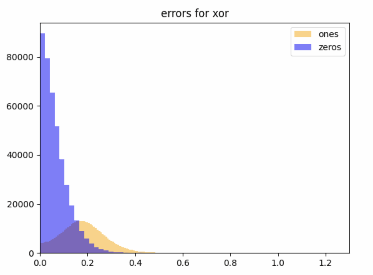
This suggests that the AND/XOR directions were -linearly readoffable at initialisation, but the evidence at this stage is weak because we don't have a good sense yet of what a reasonable value of is for considering the task to have been learned correctly: to answer this we want to fiddle around with loss functions and training for longer. For context, an affine readoff (linear + bias) directly on the inputs can read off with , which has an error of . This is larger than all but the largest errors here, and you can’t do anything like this for XOR with affine readoff.
After we did this, Kaarel came up with an argument that networks randomly initialised with weights from a standard Gaussian and zero bias solve U-AND with inputs not in superposition (although it probably can be generalised to the superposition case) for suitable readoffs. To sketch the idea:
Let be the vector of weights from the th input to the neurons. Then consider the linear readoff vector with th component given by:
where is the indicator function. There are 4 free parameters here, which are set by 4 constraints given by requiring that the expectation of this vector dotted with the activation vector has the correct value in the 4 cases . In the limit of large the value of the dot product will be very close to its expectation and we are done. There are a bunch of details to work out here and, as with the experiments, we aren't 100% sure the details all work out, but we wanted to share these new results since you asked.
A big reason to use MSE as opposed to eps-accuracy in the Anthropic model is for optimization purposes (you can't gradient descent cleanly through eps-accuracy).
We've suggested that perhaps it would be more principled to use something like loss for larger than 2, as this is closer to -accuracy. It's worth mentioning that we are currently finding that the best loss function for the task seems to be something like with extra weighting on the target values that should be . We do this to avoid the problem that if the inputs are sparse, then the ANDs are sparse too, and the model can get good loss on (for low ) by sending all inputs to the zero vector. Once we weight the ones appropriately, we find that lower values of may be better for training dynamics.
or the extension to arithmetic circuits (or other continuous/more continuous models of computation in superposition)
We agree and are keen to look into that!
(TeX compilation failure)
Thanks - fixed.