Posts
Comments
Based on the blog post, it seems like they had a system prompt that worked well enough for all of the constraints except for regexes (even though modifying the prompt to fix the regexes thing resulted in the model starting to ignore the other constraints). So it seems like the goal here was to do some custom thing to fix just the regexes (without otherwise impeding the model's performance, include performance at following the other constraints).
(Note that using SAEs to fix lots of behaviors might also have additional downsides, since you're doing a more heavy-handed intervention on the model.)
The entrypoint to their sampling code is here. It looks like they just add a forward hook to the model that computes activations for specified features and shifts model activations along SAE decoder directions a corresponding amount. (Note that this is cheaper than autoencoding the full activation. Though for all I know, running the full autoencoder during the forward pass might have been fine also, given that they're working with small models and adding a handful of SAE calls to a forward pass shouldn't be too big a hit.)
@Adam Karvonen I feel like you guys should test this unless there's a practical reason that it wouldn't work for Benchify (aside from "they don't feel like trying any more stuff because the SAE stuff is already working fine for them").
I'm guessing you'd need to rejection sample entire blocks, not just lines. But yeah, good point, I'm also curious about this. Maybe the proportion of responses that use regexes is too large for rejection sampling to work? @Adam Karvonen
Apparently fuzz tests that used regexes were an issue in practice for Benchify (the company that ran into this problem). From the blog post:
Benchify observed that the model was much more likely to generate a test with no false positives when using string methods instead of regexes, even if the test coverage wasn't as extensive.
Isn't every instance of clamping a feature's activation to 0 conditional in this sense?
x-posting a kinda rambling thread I wrote about this blog post from Tilde research.
---
If true, this is the first known application of SAEs to a found-in-the-wild problem: using LLMs to generate fuzz tests that don't use regexes. A big milestone for the field of interpretability!
I'll discussed some things that surprised me about this case study in 
---
The authors use SAE features to detect regex usage and steer models not to generate regexes. Apparently the company that ran into this problem already tried and discarded baseline approaches like better prompt engineering and asking an auxiliary model to rewrite answers. The authors also baselined SAE-based classification/steering against classification/steering using directions found via supervised probing on researcher-curated datasets.
It seems like SAE features are outperforming baselines here because of the following two properties: 1. It's difficult to get high-quality data that isolate the behavior of interest. (I.e. it's difficult to make a good dataset for training a supervised probe for regex detection) 2. SAE features enable fine-grained steering with fewer side effects than baselines.
Property (1) is not surprising in the abstract, and I've often argued that if interpretability is going to be useful, then it will be for tasks where there are structural obstacles to collecting high-quality supervised data (see e.g. the opening paragraph to section 4 of Sparse Feature Circuits https://arxiv.org/abs/2403.19647).
However, I think property (1) is a bit surprising in this particular instance—it seems like getting good data for the regex task is more "tricky and annoying" than "structurally difficult." I'd weakly guess that if you are a whiz at synthetic data generation then you'd be able to get good enough data here to train probes that outperform the SAEs. But that's not too much of a knock against SAEs—it's still cool if they enable an application that would otherwise require synthetic datagen expertise. And overall, it's a cool showcase of the fact that SAEs find meaningful units in an unsupervised way.
Property (2) is pretty surprising to me! Specifically, I'm surprised that SAE feature steering enables finer-grained control than prompt engineering. As others have noted, steering with SAE features often results in unintended side effects; in contrast, since prompts are built out of natural language, I would guess that in most cases we'd be able to construct instructions specific enough to nail down our behavior of interest pretty precisely. But in this case, it seems like the task instructions are so long and complicated that the models have trouble following them all. (And if you try to improve your prompt to fix the regex behavior, the model starts misbehaving in other ways, leading to a "whack-a-mole" problem.) And also in this case, SAE feature steering had fewer side-effects than I expected!
I'm having a hard time drawing a generalizable lesson from property (2) here. My guess is that this particular problem will go away with scale, as larger models are able to more capably follow fine-grained instructions without needing model-internals-based interventions. But maybe there are analogous problems that I shouldn't expect to be solved with scale? E.g. maybe interpretability-assisted control will be useful across scales for resisting jailbreaks (which are, in some sense, an issue with fine-grained instruction-following).
Overall, something surprised me here and I'm excited to figure out what my takeaways should be.
---
Some things that I'd love to see independent validation of:
1. It's not trivial to solve this problem with simple changes to the system prompt. (But I'd be surprised if it were: I've run into similar problems trying to engineer system prompts with many instructions.)
2. It's not trivial to construct a dataset for training probes that outcompete SAE features. (I'm at ~30% that the authors just got unlucky here.)
---
Huge kudos to everyone involved, especially the eagle-eyed @Adam Karvonen for spotting this problem in the wild and correctly anticipating that interpretability could solve it!
---
I'd also be interested in tracking whether Benchify (the company that had the fuzz-tests-without-regexes problem) ends up deploying this system to production (vs. later finding out that the SAE steering is unsuitable for a reason that they haven't yet noticed).
I've donated $5,000. As with Ryan Greenblatt's donation, this is largely coming from a place of cooperativeness: I've gotten quite a lot of value from Lesswrong and Lighthaven.[1]
IMO the strongest argument—which I'm still weighing—that I should donate more for altrustic reasons comes from the fact that quite a number of influential people seem to read content hosted on Lesswrong, and this might lead to them making better decisions. A related anecdote: When David Bau (big name professor in AI interpretability) gives young students a first intro to interpretability, his go-to example is (sometimes at least) nostalgebraist's logit lens. Watching David pull up a Lesswrong post on his computer and excitedly talk students through it was definitely surreal and entertaining.
- ^
When I was trying to assess the value I've gotten from Lightcone, I was having a hard time at first converting non-monetary value into dollars. But then I realized that there was an easy way to eyeball a monetary lower-bound for value provided me by Lightcone: estimate the effect that Lesswrong had on my personal income. Given that Lesswrong probably gets a good chunk of the credit for my career transition from academic math into AI safety research, that's a lot of dollars!
I'm quite happy for laws to be passed and enforced via the normal mechanisms. But I think it's bad for policy and enforcement to be determined by Elon Musk's personal vendettas. If Elon tried to defund the AI safety institute because of a personal vendetta against AI safety researchers, I would have some process concerns, and so I also have process concerns when these vendettas are directed against OAI.
FYI it seems like this (important-seeming) email is missing, though the surrounding emails in the exchange seem to be present. (So maybe some other ones are missing too.)
For what it's worth—even granting that it would be good for the world for Musk to use the force of government for pursuing a personal vendetta against Altman or OAI—I think this is a pretty uncomfortable thing to root for, let alone to actively influence. I think this for the same reason that I think it's uncomfortable to hope for—and immoral to contribute to—assassination of political leaders, even assuming that their assassination would be net good.
Probably I misunderstood your concern. I interpreted your concern about settings where we don't have access to ground truth as relating to cases where the model could lie about its inner states without us being able to tell (because of lack of ground truth). But maybe you're more worried about being able to develop a (sufficiently diverse) introspection training signal in the first place?
I'll also note that I'm approaching this from the angle of "does introspection have worse problems with lack-of-ground-truth than traditional interpretability?" where I think the answer isn't that clear without thinking about it more. Traditional interpretability often hill-climbs on "producing explanations that seem plausible" (instead of hill climbing on ground-truth explanations, which we almost never have access to), and I'm not sure whether this poses more of a problem for traditional interpretability vs. black-box approaches like introspection.
Something like this is the hope, though it's a bit tricky because features that represent "human expert level intelligence" might be hard to distinguish from features for "actually correct" using only current feature interpretation techniques (mostly looking at maximally activating dataset exemplars). But it seems pretty plausible that we could develop better interpretation techniques that would be suitable here.
I give a counterargument to this in the typo-riddled, poorly-written Tweet here. Sadly I won't have a chance to write up thoughts here more cleanly for a few days.
ETA: Briefly, the key points are:
- Honesty issues for introspection aren't obviously much worse than they are for simple probing. (But fair if you're already not excited about simple probing.)
- When you can ask models arbitrary questions about their cognition, I think it's probably quite difficult for a model to tell on which inputs it can get away with lying.
While I agree the example in Sycophancy to Subterfuge isn't realistic, I don't follow how the architecture you describe here precludes it. I think a pretty realistic set-up for training an agent via RL would involve computing scalar rewards on the execution machine or some other machine that could be compromised from the execution machine (with the scalar rewards being sent back to the inference machine for backprop and parameter updates).
I continue to think that capabilities from in-context RL are and will be a rounding error compared to capabilities from training (and of course, compute expenditure in training has also increased quite a lot in the last two years).
I do think that test-time compute might matter a lot (e.g. o1), but I don't expect that things which look like in-context RL are an especially efficient way to make use of test-time compute.
Why would it 2x the cost of inference? To be clear, my suggested baseline is "attach exactly the same LoRA adapters that were used for RR, plus one additional linear classification head, then train on an objective which is similar to RR but where the rerouting loss is replaced by a classification loss for the classification head." Explicitly this is to test the hypothesis that RR only worked better than HP because it was optimizing more parameters (but isn't otherwise meaningfully different from probing).
(Note that LoRA adapters can be merged into model weights for inference.)
(I agree that you could also just use more expressive probes, but I'm interested in this as a baseline for RR, not as a way to improve robustness per se.)
Thanks to the authors for the additional experiments and code, and to you for your replication and write-up!
IIUC, for RR makes use of LoRA adapters whereas HP is only a LR probe, meaning that RR is optimizing over a more expressive space. Does it seem likely to you that RR would beat an HP implementation that jointly optimizes LoRA adapters + a linear classification head (out of some layer) so that the model retains performance while also having the linear probe function as a good harmfulness classifier?
(It's been a bit since I read the paper, so sorry if I'm missing something here.)
Anthropic has asked employees
[...]
Anthropic has offered at least one employee
As a point of clarification: is it correct that the first quoted statement above should be read as "at least one employee" in line with the second quoted statement? (When I first read it, I parsed it as "all employees" which was very confusing since I carefully read my contract both before signing and a few days ago (before posting this comment) and I'm pretty sure there wasn't anything like this in there.)
(I'm a full-time employee at Anthropic.) It seems worth stating for the record that I'm not aware of any contract I've signed whose contents I'm not allowed to share. I also don't believe I've signed any non-disparagement agreements. Before joining Anthropic, I confirmed that I wouldn't be legally restricted from saying things like "I believe that Anthropic behaved recklessly by releasing [model]".
there are multiple possible ways to interpret the final environment in the paper in terms of the analogy to the future:
- As the catastrophic failure that results from reward hacking. In this case, we might care about frequency depending on the number of opportunities the model would have and the importance of collusion.
You're correct that I was neglecting this threat model—good point, and thanks.
So, given this overall uncertainty, it seems like we should have a much fuzzier update where higher numbers should actually update us.
Hmm, here's another way to frame this discussion:
Sam: Before evaluating the RTFs in the paper, you should apply a ~sigmoid function with the transition region centered on ~10^-6 or something. Note that all of the RTFs we're discussing come after this transition.
Ryan: While it's true that we should first be applying a ~sigmoid, we should have uncertainty over where the transition region begins. When taking this uncertainty into account, the way to decide importance boils down to comparing the observed RTF to your distribution of thresholds in a way which is pretty similar to what people were implicitly doing anyway.
Does that sound like a reasonable summary? If so, I think I basically agree with you.
(I do think that it's important to keep in mind that for threat models where reward hacking is reinforced, small RTFs might matter a lot, but maybe that was already obvious to everyone.)
In this comment, I'll use reward tampering frequency (RTF) to refer to the proportion of the time the model reward tampers.
I think that in basically all of the discussion above, folks aren't using a correct mapping of RTF to practical importance. Reward hacking behaviors are positively reinforced once they occur in training; thus, there's a rapid transition in how worrying a given RTF is, based on when reward tampering becomes frequent enough that it's likely to appear during a production RL run.
To put this another way: imagine that this paper had trained on the final reward tampering environment the same way that it trained on the other environments. I expect that:
- the RTF post-final-training-stage would be intuitively concerning to everyone
- the difference between 0.01% and 0.02% RTF pre-final-training-stage wouldn't have a very big effect on RTF post-final-training-stage.
In other words, insofar as you're updating on this paper at all, I think you should be updating based on whether the RTF > 10^-6 (not sure about the exact number, but something like this) and the difference between RTFs of 1e-4 and 2e-4 just doesn't really matter.
Separately, I think it's also defensible to not update much on this paper because it's very unlikely that AI developers will be so careless as to allow models they train a chance to directly intervene on their reward mechanism. (At least, not unless some earlier thing has gone seriously wrong.) (This is my position.)
Anyway, my main point is that if you think the numbers in this paper matter at all, it seems like they should matter in the direction of being concerning. [EDIT: I mean this in the sense of "If reward tampering actually occurred with this frequency in training of production models, that would be very bad." Obviously for deciding how to update you should be comparing against your prior expectations.]
This was awesome. Here are some more stories in the same style.
Homeless person or professor?
It can be hard to tell in Cambridge, Massachusetts. That's partly because some professors—mostly the MIT ones—can look very disheveled. But partly it's because some homeless people can be surprisingly intellectual, e.g. it's not uncommon to find homeless people crouched in the shade reading a book.
My favorite example is a homeless man in Harvard Square. His name in my head is "Black Santa" because he's a old man with a full belly and white beard, and he's always surrounded by trash-bag-sacks not of toys, but of his possessions. He's always in the same spot, a stretch of Harvard Square that lots of homeless people hang out in. But while the other, mostly young, homeless in the area typically spend their time begging or zonked out, I only ever see Black Santa writing in a small notebook.
What's he writing all the time? As best I can tell from peeping over his shoulder as I pass by, he's writing poetry. Sometimes I spot him reciting it out loud before he goes back to scribbling.
Some day I hope to muster the courage to strike up a conversation out of the blue with him and learn more.
Remember that time I broke all my limbs at once...?
Most of my chats with homeless people happened when I had a fractured leg and was moving around in crutches. I think for the local homeless people—many of whom have disabilities, and essentially all of whom have friends with disabilities—the crutches made me seem more familiar. Or maybe it was just that I was spending more time sitting at bus stops with nothing to do but talk.
The most interesting, and the saddest, conversation I had was with a man who recognized my knee brace: "oh yeah I had one of those once too. Two of them actually."
"Did you break your leg twice? I'm sorry."
"Well, two of them at the same time I mean—both my legs were broken. Both my arms too. I got hit by a car and it broke both my arms and legs."
"Oh god, that's horrible."
"Yeah the medical bill was rough, no way I could pay it. I heard an ad on the radio for one of those lawyers that sues people for stuff like this. So I hired them and sued the person who hit me."
"Did you win?"
"Yeah, but the person who hit me didn't have any money, so I didn't actually get anything out of it..."
If something like this had happened to me, I think it would be the most traumatic event of my life, one that hurt to remember. On the other hand, the man telling the story told it casually, as if he kept remembering more things he did over the weekend that he wanted to chat about.
Would you like some cheese?
There's a kindly alcoholic that I sometimes see at the bus stop outside my apartment. He often smiles at me and says hello when I go by.
The first time I saw him, he was sitting there with a huge plastic-wrapped wedge of Jarlsberg cheese. With a giddy grin, he held it out to me in offering. I do like Jarlsberg, but declined.
An hour later I left my apartment and the man was gone. In his place was the unwrapped wedge of cheese on the ground with a single bite taken out of it.
I should have accepted the cheese!
I think this is cool! The way I'm currently thinking about this is "doing the adversary generation step of latent adversarial training without the adversarial training step." Does that seem right?
It seems intuitively plausible to me that once you have a latent adversarial perturbation (the vectors you identify), you might be able to do something interesting with it beyond "train against it" (as LAT does). E.g. maybe you would like to know that your model has a backdoor, beyond wanting to move to the next step of "train away the backdoor." If I were doing this line of work, I would try to some up with toy scenarios with the property "adversarial examples are useful for reasons other than adversarial training" and show that the latent adversarial examples you can produce are more useful than input-level adversarial examples (in the same way that the LAT paper demonstrates that LAT can outperform input-level AT).
Yep, you're totally right -- thanks!
Oh, one other issue relating to this: in the paper it's claimed that if is the argmin of then is the argmin of . However, this is not actually true: the argmin of the latter expression is . To get an intuition here, consider the case where and are very nearly perpendicular, with the angle between them just slightly less than . Then you should be able to convince yourself that the best factor to scale either or by in order to minimize the distance to the other will be just slightly greater than 0. Thus the optimal scaling factors cannot be reciprocals of each other.
ETA: Thinking on this a bit more, this might actually reflect a general issue with the way we think about feature shrinkage; namely, that whenever there is a nonzero angle between two vectors of the same length, the best way to make either vector close to the other will be by shrinking it. I'll need to think about whether this makes me less convinced that the usual measures of feature shrinkage are capturing a real thing.
ETA2: In fact, now I'm a bit confused why your figure 6 shows no shrinkage. Based on what I wrote above in this comment, we should generally expect to see shrinkage (according to the definition given in equation (9)) whenever the autoencoder isn't perfect. I guess the answer must somehow be "equation (10) actually is a good measure of shrinkage, in fact a better measure of shrinkage than the 'corrected' version of equation (10)." That's pretty cool and surprising, because I don't really have a great intuition for what equation (10) is actually capturing.
Ah thanks, you're totally right -- that mostly resolves my confusion. I'm still a little bit dissatisfied, though, because the term is optimizing for something that we don't especially want (i.e. for to do a good job of reconstructing ). But I do see how you do need to have some sort of a reconstruction-esque term that actually allows gradients to pass through to the gated network.
(The question in this comment is more narrow and probably not interesting to most people.)
The limitations section includes this paragraph:
One worry about increasing the expressivity of sparse autoencoders is that they will overfit when
reconstructing activations (Olah et al., 2023, Dictionary Learning Worries), since the underlying
model only uses simple MLPs and attention heads, and in particular lacks discontinuities such as step
functions. Overall we do not see evidence for this. Our evaluations use held-out test data and we
check for interpretability manually. But these evaluations are not totally comprehensive: for example,
they do not test that the dictionaries learned contain causally meaningful intermediate variables in the
model’s computation. The discontinuity in particular introduces issues with methods like integrated
gradients (Sundararajan et al., 2017) that discretely approximate a path integral, as applied to SAEs
by Marks et al. (2024).
I'm not sure I understand the point about integrated gradients here. I understand this sentence as meaning: since model outputs are a discontinuous function of feature activations, integrated gradients will do a bad job of estimating the effect of patching feature activations to counterfactual values.
If that interpretation is correct, then I guess I'm confused because I think IG actually handles this sort of thing pretty gracefully. As long as the number of intermediate points you're using is large enough that you're sampling points pretty close to the discontinuity on both sides, then your error won't be too large. This is in contrast to attribution patching which will have a pretty rough time here (but not really that much worse than with the normal ReLU encoders, I guess). (And maybe you also meant for this point to apply to attribution patching?)
I'm a bit perplexed by the choice of loss function for training GSAEs (given by equation (8) in the paper). The intuitive (to me) thing to do here would be would be to have the and terms, but not the term, since the point of is to tell you which features should be active, not to itself provide good feature coefficients for reconstructing . I can sort of see how not including this term might result in the coordinates of all being extremely small (but barely positive when it's appropriate to use a feature), such that the sparsity term doesn't contribute much to the loss. Is that what goes wrong? Are there ablation experiments you can report for this? If so, including this term still currently seems to me like a pretty unprincipled way to deal with this -- can the authors provide any flavor here?
Here are two ways that I've come up with for thinking about this loss function -- let me know if either of these are on the right track. Let denote the gated encoder, but with a ReLU activation instead of Heaviside. Note then that is just the standard SAE encoder from Towards Monosemanticity.
Perspective 1: The usual loss from Towards Monosemanticity for training SAEs is (this is the same as your and up to the detaching thing). But now you have this magnitude network which needs to get a gradient signal. Let's do that by adding an additional term -- your . So under this perspective, it's the reconstruction term which is new, with the sparsity and auxiliary terms being carried over from the usual way of doing things.
Perspective 2 (h/t Jannik Brinkmann): let's just add together the usual Towards Monosemanticity loss function for both the usual architecture and the new modified archiecture: .
However, the gradients with respect to the second term in this sum vanish because of the use of the Heaviside, so the gradient with respect to this loss is the same as the gradient with respect to the loss you actually used.
I believe that equation (10) giving the analytical solution to the optimization problem defining the relative reconstruction bias is incorrect. I believe the correct expression should be .
You could compute this by differentiating equation (9), setting it equal to 0 and solving for . But here's a more geometrical argument.
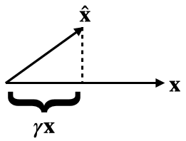
By definition, is the multiple of closest to . Equivalently, this closest such vector can be described as the projection . Setting these equal, we get the claimed expression for .
As a sanity check, when our vectors are 1-dimensional, , and , we my expression gives (which is correct), but equation (10) in the paper gives .
Great work! Obviously the results here speak for themselves, but I especially wanted to complement the authors on the writing. I thought this paper was a pleasure to read, and easily a top 5% exemplar of clear technical writing. Thanks for putting in the effort on that.
I'll post a few questions as children to this comment.
I'm pretty sure that you're not correct that the interpretation step from our SHIFT experiments essentially relies on using data from the Pile. I strongly expect that if we were to only use inputs from then we would be able to interpret the SAE features about as well. E.g. some of the SAE features only activate on female pronouns, and we would be able to notice this. Technically, we wouldn't be able to rule out the hypothesis "this feature activates on female pronouns only when their antecedent is a nurse," but that would be a bit of a crazy hypothesis anyway.
In more realistic settings (larger models and subtler behaviors) we might have more serious problems ruling out hypotheses like this. But I don't see any fundamental reason that using disambiguating datapoints is strictly necessary.
(Edits made. In the edited version, I think the only questionable things are the title and the line "[In this post, I will a]rticulate a class of approaches to scalable oversight I call cognition-based oversight." Maybe I should be even more careful and instead say that cognition-based oversight is merely something that "could be useful for scalable oversight," but I overall feel okay about this.
Everywhere else, I think the term "scalable oversight" is now used in the standard way.)
I (mostly; see below) agree that in this post I used the term "scalable oversight" in a way which is non-standard and, moreover, in conflict way the way I typically use the term personally. I also agree with the implicit meta-point that it's important to be careful about using terminology in a consistent way (though I probably don't think it's as important as you do). So overall, after reading this comment, I wish I had been more careful about how I treated the term "scalable oversight." After I post this comment, I'll make some edits for clarity, but I don't expect to go so far as to change the title[1].
Two points in my defense:
- Even though "scalable oversight" isn't an appropriate description for the narrow technical problem I pose here, the way I expect progress on this agenda to actually get applied is well-described as scalable oversight.
- I've found the scalable oversight frame on this problem useful both for my own thinking about it and for explaining it to others.
Re (1): I spend most of my time thinking about the sycophantic reward hacking threat model. So in my head, some of the model's outputs really are bad but it's hard to notice this. Here are two ways that I think this agenda could help with noticing bad particular outputs:
- By applying DBIC to create classifiers for particular bad things (e.g. measurement tampering) which we apply to detect bad outputs.
- By giving us a signal about which episodes should be more closely scrutinized, and which aspects of those episodes we should scrutinize. (For example, suppose you notice that your model is thinking about a particular camera in a maybe-suspicious way, so you look for tricky ways that that camera could have been tampered with, and after a bunch of targeted scrutiny you notice a hack).
I think that both of these workflows are accurately described as scalable oversight.
Re (2): when I explain that I want to apply interpretability to scalable oversight, people -- including people that I really expected to know better -- often react with surprise. This isn't, I think, because they're thinking carefully about what scalable oversight means the way that you are. Rather, it seems that a lot of people split alignment work into two non-interacting magisteria called "scalable oversight" and "solving deceptive alignment," and they classify interpretability work as being part of the latter magisterium. Such people tend to not realize that e.g. ELK is centrally a scalable oversight agenda, and I think of my proposed agenda here as attempting to make progress on ELK (or on special cases thereof).
I guess my post muddies the water on all of the above by bringing up scheming; even though this technically fits into the setting I propose to make progress on, I don't really view it as the central problem I'm trying to solve.
- ^
Sadly, if I say that my goal is to use interpretability to "evaluate models" then I think people will pattern-match this to "evals" which typically means something different, e.g. checking for dangerous capabilities. I can't really think of a better, non-confusing term for the task of "figuring out whether a model is good or bad." Also, I expect that the ways progress on this agenda will actually be applied do count as "scalable oversight"; see below.
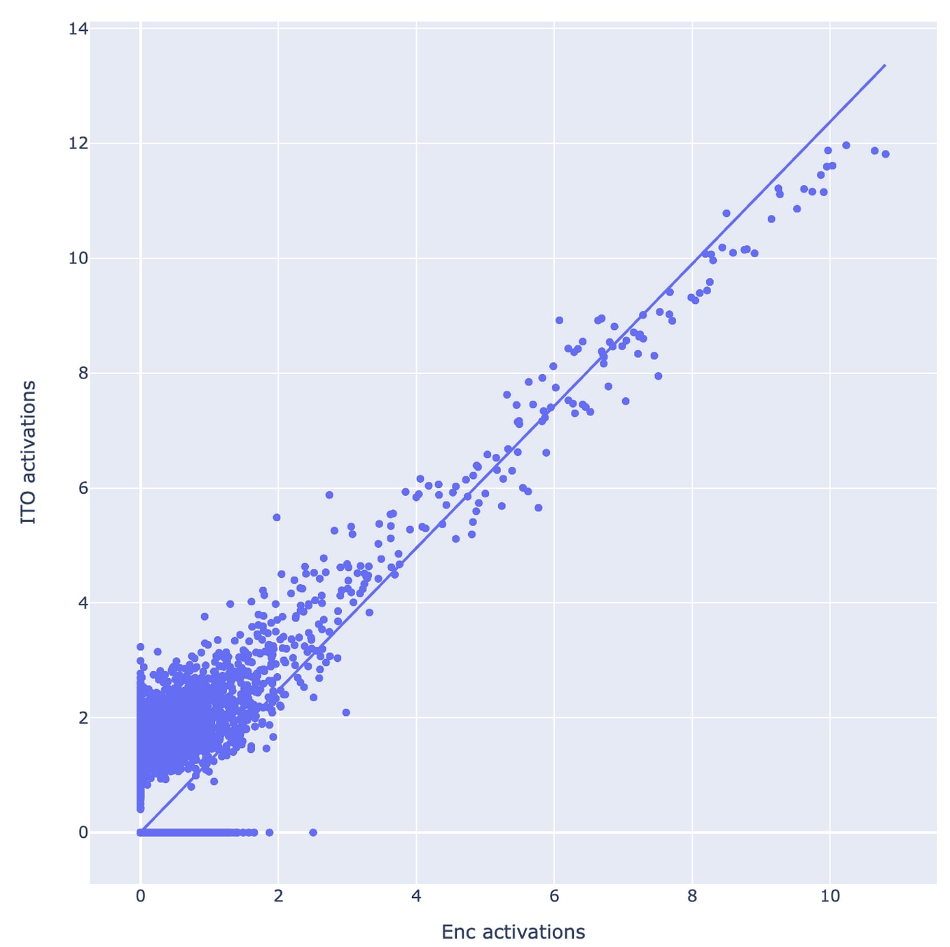
With the ITO experiments, my first guess would be that reoptimizing the sparse approximation problem is mostly relearning the encoder, but with some extra uninterpretable hacks for low activation levels that happen to improve reconstruction. In other words, I'm guessing that the boost in reconstruction accuracy (and therefore loss recovered) is mostly not due to better recognizing the presence of interpretable features, but by doing fiddly uninterpretable things at low activation levels.
I'm not really sure how to operationalize this into a prediction. Maybe something like: if you pick some small-ish threshold T (maybe like T=3 based on the plot copied below) and round activations less than T down to 0 (for both the ITO encoder and the original encoder), then you'll no longer see that the ITO encoder outperforms the original one.
Awesome stuff -- I think that updates like this (both from the GDM team and from Anthropic) are very useful for organizing work in this space. And I especially appreciate the way this was written, with both short summaries and in-depth write-ups.
I originally ran some of these experiments on 7B and got very different results, that PCA plot of 7B looks familiar (and bizarre).
I found that the PCA plot for 7B for larger_than and smaller_than individually looked similar to that for 13B, but that the PCA plot for larger_than + smaller_than looked degenerate in the way I screenshotted. Are you saying that your larger_than + smaller_than PCA looked familiar for 7B?
I suppose there are two things we want to separate: "truth" from likely statements, and "truth" from what humans think (under some kind of simulacra framing). I think this approach would allow you to do the former, but not the latter. And to be honest, I'm not confident on TruthfulQA's ability to do the latter either.
Agreed on both points.
We differ slightly from the original GoT paper in naming, and use
got_citiesto refer to both thecitiesandneg_citiesdatasets. The same is true forsp_en_transandlarger_than. We don't do this forcities_cities_{conj,disj}and leave them unpaired.
Thanks for clarifying! I'm guessing this is what's making the GoT datasets much worse for generalization (from and to) in your experiments. For 13B, it mostly seemed to me that training on negated statements helped for generalization to other negated statements, and that pairing negated statements with unnegated statements in training data usually (but not always) made generalization to unnegated datasets a bit worse. (E.g. the cities -> sp_en_trans generalization is better than cities + neg_cities -> sp_en_trans generalization.)
Very cool! Always nice to see results replicated and extended on, and I appreciated how clear you were in describing your experiments.
Do smaller models also have a generalised notion of truth?
In my most recent revision of GoT[1] we did some experiments to see how truth probe generalization changes with model scale, working with LLaMA-2-7B, -13B, and -70B. Result: truth probes seems to generalize better for larger models. Here are the relevant figures.
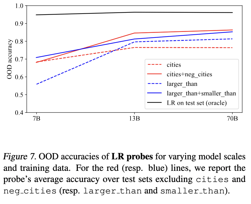
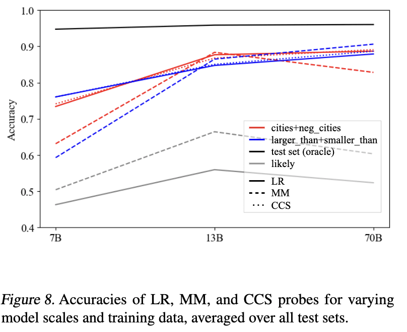
Some other related evidence from our visualizations:
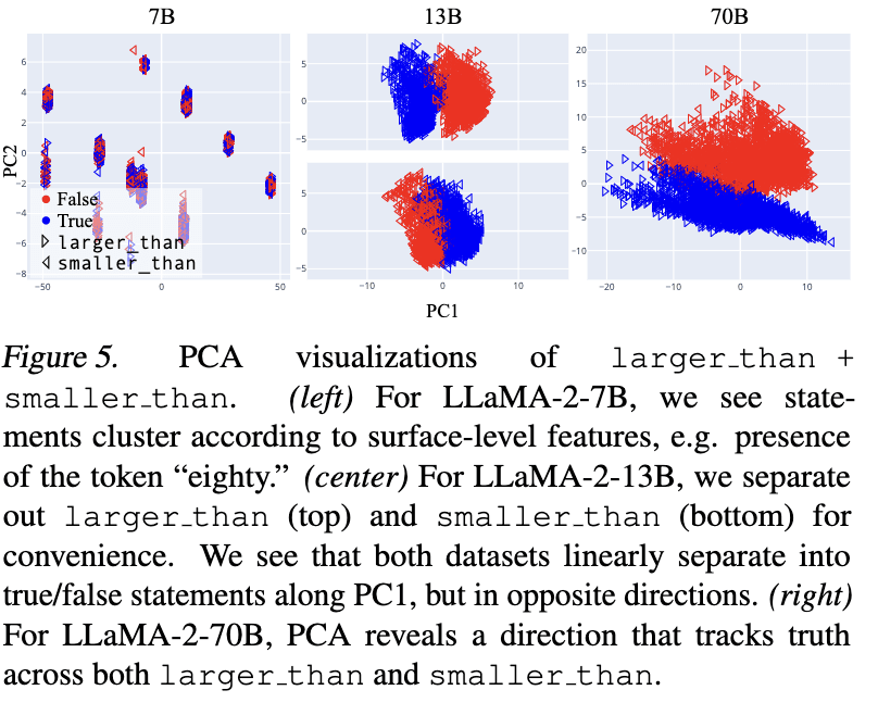
We summed things up like so, which I'll just quote in its entirety:
Overall, these visualizations suggest a picture like the following: as LLMs scale (and perhaps, also as a fixed LLM progresses through its forward pass), they hierarchically develop and linearly represent increasingly general abstractions. Small models represent surface-level characteristics of their inputs; these surface-level characteristics may be sufficient for linear probes to be accurate on narrow training distributions, but such probes are unlikely to generalize out-of-distribution. Large models linearly represent more abstract concepts, potentially including abstract notions like “truth” which capture shared properties of topically and structurally diverse inputs. In middle regimes, we may find linearly represented concepts of intermediate levels of abstraction, for example, “accurate factual recall” or “close association” (in the sense that “Beijing” and “China” are closely associated). These concepts may suffice to distinguish true/false statements on individual datasets, but will only generalize to test data for which the same concepts
suffice.
How do we know we’re detecting truth, and not just likely statements?
One approach here is to use a dataset in which the truth and likelihood of inputs are uncorrelated (or negatively correlated), as you kinda did with TruthfulQA. For that, I like to use the "neg_" versions of the datasets from GoT, containing negated statements like "The city of Beijing is not in China." For these datasets, the correlation between truth value and likelihood (operationalized as LLaMA-2-70B's log probability of the full statement) is strong and negative (-0.63 for neg_cities and -.89 for neg_sp_en_trans). But truth probes still often generalize well to these negated datsets. Here are results for LLaMA-2-70B (the horizontal axis shows the train set, and the vertical axis shows the test set).
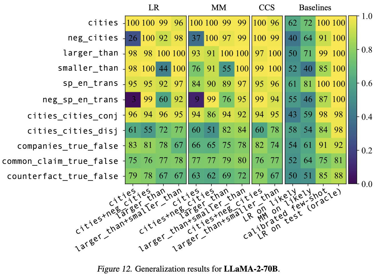
We also find that the probe performs better than LDA in-distribution, but worse out-of-distribution:
Yep, we found the same thing -- LDA improves things in-distribution, but generalizes work than simple DIM probes.
Why does got_cities_cities_conj generalise well?
I found this result surprising, thanks! I don't really have great guesses for what's going on. One thing I'll say is that it's worth tracking differences between various sorts of factual statements. For example, for LLaMA-2-13B it generally seemed to me that there was better probe transfer between factual recall datasets (e.g. cities and sp_en_trans, but not larger_than). I'm not really sure why the conjunctions are making things so much better, beyond possibly helping to narrow down on "truth" beyond just "correct statement of factual recall."
I'm not surprised that cities_cities_conj and cities_cities_disj are so qualitatively different -- cities_cities_disj has never empirically played well with the other datasets (in the sense of good probe transfer) and I don't really know why.
This comment is about why we were getting different MSE numbers. The answer is (mostly) benign -- a matter of different scale factors. My parallel comment, which discusses why we were getting different CE diff numbers is the more important one.
When you compute MSE loss between some activations and their reconstruction , you divide by variance of , as estimated from the data in a batch. I'll note that this doesn't seem like a great choice to me. Looking at the resulting training loss:
where is the encoding of by the autoencoder and is the L1 regularization constant, we see that if you scale by some constant , this will have no effect on the first term, but will scale the second term by . So if activations generically become larger in later layers, this will mean that the sparsity term becomes automatically more strongly weighted.
I think a more principled choice would be something like
where we're no longer normalizing by the variance, and are also using sqrt(MSE) instead of MSE. (This is what the dictionary_learning repo does.) When you scale by a constant , this entire expression scales by a factor of , so that the balance between reconstruction and sparsity remains the same. (On the other hand, this will mean that you might need to scale the learning rate by , so perhaps it would be reasonable to divide through this expression by ? I'm not sure.)
Also, one other thing I noticed: something which we both did was to compute MSE by taking the mean over the squared difference over the batch dimension and the activation dimension. But this isn't quite what MSE usually means; really we should be summing over the activation dimension and taking the mean over the batch dimension. That means that both of our MSEs are erroneously divided by a factor of the hidden dimension (768 for you and 512 for me).
This constant factor isn't a huge deal, but it does mean that:
- The MSE losses that we're reporting are deceptively low, at least for the usual interpretation of "mean squared error"
- If we decide to fix this, we'll need to both scale up our L1 regularization penalty by a factor of the hidden dimension (and maybe also scale down the learning rate).
This is a good lesson on how MSE isn't naturally easy to interpret and we should maybe just be reporting percent variance explained. But if we are going to report MSE (which I have been), I think we should probably report it according to the usual definition.
Yep, as you say, @Logan Riggs figured out what's going on here: you evaluated your reconstruction loss on contexts of length 128, whereas I evaluated on contexts of arbitrary length. When I restrict to context length 128, I'm able to replicate your results.
Here's Logan's plot for one of your dictionaries (not sure which)
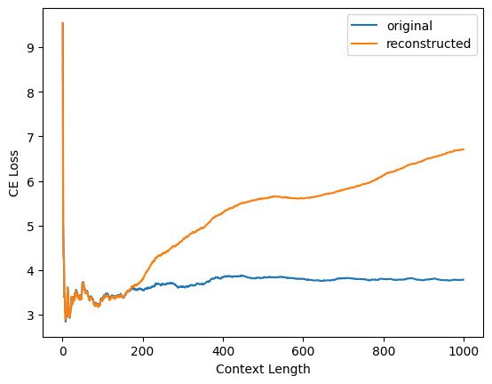
and here's my replication of Logan's plot for your layer 1 dictionary
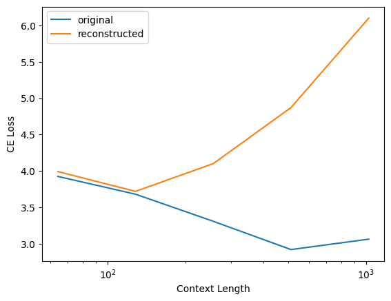
Interestingly, this does not happen for my dictionaries! Here's the same plot but for my layer 1 residual stream output dictionary for pythia-70m-deduped

(Note that all three plots have a different y-axis scale.)
Why the difference? I'm not really sure. Two guesses:
- The model: GPT2-small uses learned positional embeddings whereas Pythia models use rotary embeddings
- The training: I train my autoencoders on variable-length sequences up to length 128; left padding is used to pad shorter sequences up to length 128. Maybe this makes a difference somehow.
In terms of standardization of which metrics to report, I'm torn. On one hand, for the task your dictionaries were trained on (reconstruction activations taken from length 128 sequences), they're performing well and this should be reflected in the metrics. On the other hand, people should be aware that if they just plug your autoencoders into GPT2-small and start doing inference on inputs found in the wild, things will go off the rails pretty quickly. Maybe the answer is that CE diff should be reported both for sequences of the same length used in training and for arbitrary-length sequences?
My SAEs also have a tied decoder bias which is subtracted from the original activations. Here's the relevant code in dictionary.py
def encode(self, x):
        return nn.ReLU()(self.encoder(x - self.bias))

    def decode(self, f):
        return self.decoder(f) + self.bias

    def forward(self, x, output_features=False, ghost_mask=None):
            [...]
            f = self.encode(x)
            x_hat = self.decode(f)
            [...]
            return x_hat
Note that I checked that our SAEs have the same input-output behavior in my linked colab notebook. I think I'm a bit confused why subtracting off the decoder bias had to be done explicitly in your code -- maybe you used dictionary.encoder and dictionary.decoder instead of dictionary.encode and dictionary.decode? (Sorry, I know this is confusing.) ETA: Simple things I tried based on the hypothesis "one of us needs to shift our inputs by +/- the decoder bias" only made things worse, so I'm pretty sure that you had just initially converted my dictionaries into your infrastructure in a way that messed up the initial decoder bias, and therefore had to hand-correct it.
I note that the MSE Loss you reported for my dictionary actually is noticeably better than any of the MSE losses I reported for my residual stream dictionaries! Which layer was this? Seems like something to dig into.
At the time that I made this post, no, but this has been implemented in dictionary_learning since I saw your suggestion to do so in your linked post.
Another sanity check: when you compute CE loss using the same code that you use when computing CE loss when activations are reconstructed by the autoencoders, but instead of actually using the autoencoder you just plug the correct activations back in, do you get the same answer (~3.3) as when you evaluate CE loss normally?
In the notebook I link in my original comment, I check that the activations I get out of nnsight are the same as the activations that come from transformer_lens. Together with the fact that our sparsity statistics broadly align, I'm guessing that the issue isn't that I'm extracting different activations than you are.
Repeating my replication attempt with data from OpenWebText, I get this:
| Layer | MSE Loss | % Variance Explained | L1 | L0 | % Alive | CE Reconstructed |
|---|---|---|---|---|---|---|
| 1 | 0.069 | 95 | 40 | 15 | 46 | 6.45 |
| 7 | 0.81 | 86 | 125 | 59.2 | 96 | 4.38 |
Broadly speaking, same story as above, except that the MSE losses look better (still not great), and that the CE reconstructed looks very bad for layer 1.
I don't much padding at all, that might be a big difference too.
Seems like there was a typo here -- what do you mean?
Logan Riggs reports that he tried to replicate your results and got something more similar to you. I think Logan is making decisions about padding and tokenization more like the decisions you make, so it's possible that the difference is down to something around padding and tokenization.
Possible next steps:
- Can you report your MSE Losses (instead of just variance explained)?
- Can you try to evaluate the residual stream dictionaries in the 5_32768 set released here? If you get CE reconstructed much better than mine, then it means that we're computing CE reconstructed in different ways, where your way consistently reports better numbers. If you get CE reconstructed much worse than mine, then it might mean that there's a translation error between our codebases (e.g. using different activations).
I tried replicating your statistics using my own evaluation code (in evaluation.py here). I pseudo-randomly chose layer 1 and layer 7. Sadly, my results look rather different from yours:
| Layer | MSE Loss | % Variance Explained | L1 | L0 | % Alive | CE Reconstructed |
|---|---|---|---|---|---|---|
| 1 | 0.11 | 92 | 44 | 17.5 | 54 | 5.95 |
| 7 | 1.1 | 82 | 137 | 65.4 | 95 | 4.29 |
Places where our metrics agree: L1 and L0.
Places where our metrics disagree, but probably for a relatively benign reason:
- Percent variance explained: my numbers are slightly lower than yours, and from a brief skim of your code I think it's because you're calculating variance slightly incorrectly: you're not subtracting off the activation's mean before doing .pow(2).sum(-1). This will slightly overestimate the variance of the original activations, so probably also overestimate percent variance explained.
- Percent alive: my numbers are slightly lower than yours, and this is probably because I determined whether neurons are alive on a (somewhat small) batch of 8192 tokens. So my number is probably an underestimate and yours is correct.
Our metrics disagree strongly on CE reconstructed, and this is a bit alarming. It means that either you have a bug which significantly underestimates reconstructed CE loss, or I have a bug which significantly overestimates it. I think I'm 50/50 on which it is. Note that according to my stats, your MSE loss is kinda bad, which would suggest that you should also have high CE reconstructed (especially when working with residual stream dictionaries! (in contrast to e.g. MLP dictionaries which are much more forgiving)).
Spitballing a possible cause: when computing CE loss, did you exclude padding tokens? If not, then it's possible that many of the tokens on which you're computing CE are padding tokens, which is artificially making your CE look extremely good.
Here is my code. You'll need to pip install nnsight before running it. Many thanks to Caden Juang for implementing the UnifiedTransformer functionality in nnsight, which is a crazy Frankenstein marriage of nnsight and transformer_lens; it would have been very hard for me to attempt this replication without this feature.
Some updates about the dictionary_learning repo:
- The repo now has support for ghost grads. h/t g-w1 for submitting a PR for this
ActivationBuffersnow work natively with model components -- like the residual stream -- whose activations are typically returned as tuples; the buffer knows to take the first component of the tuple (and will iteratively do this if working with nested tuples).ActivationBufferscan now be stored on the GPU.- The file
evaluation.pycontains code for evaluating trained dictionaries. I've found this pretty useful for quickly evaluating dictionaries people send to me. - New convenience: you can do
reconstructed_acts, features = dictionary(acts, output_features=True)to get both the reconstruction and the features computed bydictionary.
Also, if you'd like to train dictionaries for many model components in parallel, you can use the parallel branch. I don't promise to never make breaking changes to the parallel branch, sorry.
Finally, we've released a new set of dictionaries for the MLP outputs, attention outputs, and residual stream in all layers of Pythia-70m-deduped. The MLP and attention dictionaries seem pretty good, and the residual stream dictionaries seem like a mixed bag. Their stats can be found here.
Thanks, I've disliked the shoggoth meme for a while, and this post does a better job articulating why than I've been able to do myself.
Imo "true according to Alice" is nowhere near as "crazy" a feature as "has_true XOR has_banana". It seems useful for the LLM to model what is true according to Alice! (Possibly I'm misunderstanding what you mean by "crazy" here.)
I agree with this! (And it's what I was trying to say; sorry if I was unclear.) My point is that
{ features which are as crazy as "true according to Alice" (i.e., not too crazy)}
seems potentially manageable, where as
{ features which are as crazy as arbitrary boolean functions of other features }
seems totally unmanageable.
Thanks, as always, for the thoughtful replies.
Idk, I think it's pretty hard to know what things are and aren't useful for predicting the next token. For example, some of your features involve XORing with a "has_not" feature -- XORing with an indicator for "not" might be exactly what you want to do to capture the effect of the "not".
I agree that "the model has learned the algorithm 'always compute XORs with has_not'" is a pretty sensible hypothesis. (And might be useful to know, if true!) FWIW, the stronger example of "clearly not useful XORs" I was thinking of has_true XOR has_banana, where I'm guessing you're anticipating that this XOR exists incidentally.
If you want you could rephrase this issue as " and are spuriously correlated in training," so I guess I should say "even in the absence of spurious correlations among basic features."
... That's exactly how I would rephrase the issue and I'm not clear on why you're making a sharp distinction here.
Focusing again on the Monster gridworld setting, here are two different ways that your goals could misgeneralize:
- player_has_shield is spuriously correlated with high_score during training, so the agent comes to value both
- monster_present XOR high_score is spuriously correlated with high_score during training, so the agent comes to value both.
These are pretty different things that could go wrong. Before realizing that these crazy XOR features existed, I would only have worried about (1); now that I know these crazy XOR features exist ... I think I mostly don't need to worry about (2), but I'm not certain and it might come down to details about the setting. (Indeed, your CCS challenges work has shown that sometimes these crazy XOR features really can get in the way!)
I agree that you can think of this issue as just being the consequence of the two issues "there are lots of crazy XOR features" and "linear probes can pick up on spurious correlations," I guess this issue feels qualitatively new to me because it just seems pretty untractable to deal with it on the data augmentation level (how do you control for spurious correlations with arbitrary boolean functions of undesired features?). I think you mostly need to hope that it doesn't matter (because the crazy XOR directions aren't too salient) or come up with some new idea.
I'll note that if it ends up these XOR directions don't matter for generalization in practice, then I start to feel better about CCS (along with other linear probing techniques).[1]
my main claim is that it shouldn't be surprising
If I had to articulate my reason for being surprised here, it'd be something like:
- I didn't expect LLMs to compute many XORs incidentally
- I didn't expect LLMs to compute many XORs because they are useful
but lots of XORs seem to get computed anyway. So at least one of these two mechanisms is occurring a surprising (to me) amount. If there's a lot more incidental computation, then why? (Based on Fabian's experiments, maybe the answer is "there's more redundancy than I expected," which would be interesting.) If there's a lot more intentional computation of XORs than I expected, then why? (I've found the speculation that LLMs might just computing a bunch of XORs up front because they don't know what they'll need later interesting.) I could just update my world model to "lots of XORs exist for either reasons (1) or (2)," but I sure would be interested in knowing which of (1) or (2) it is and why.
- ^
I know that for CCS you're more worried about issues around correlations with features like true_according_to_Alice, but my feeling is that we might be able to handle spurious features that are that crazy and numerous, but not spurious features as crazy and numerous as these XORs.
I agree with a lot of this, but some notes:
Exponentially many features
[...]
On utility explanations, you would expect that multi-way XORs are much less useful for getting low loss than two-way XORs, and so computation for multi-way XORs is never developed.
The thing that's confusing here is that the two-way XORs that my experiments are looking at just seem clearly not useful for anything. So I think any utility explanation that's going to be correct needs to be a somewhat subtle one of the form "the model doesn't initially know which XORs will be useful, so it just dumbly computes way more XORs than it needs, including XORs which are never used in any example in training." Or in other words "the model has learned the algorithm 'compute lots of XORs' rather than having learned specific XORs which it's useful to compute."
I think this subtlety changes the story a bit. One way that it changes the story is that you can't just say "the model won't compute multi-way XORs because they're not useful" -- the two-way XORs were already not useful! You instead need to argue that the model is implementing an algorithm which computed all the two-way XORs but didn't compute XORs of XORs; it seems like this algorithm might need to encode somewhere information about which directions correspond to basic features and which don't.
On the other hand, RAX introduces a qualitatively new way that linear probes can fail to learn good directions. Suppose a is a feature you care about (e.g. “true vs. false statements”) and b is some unrelated feature which is constant in your training data (e.g. b = “relates to geography”). [...]
Fwiw, failures like this seem plausible without RAX as well. We explicitly make this argument in our goal misgeneralization paper (bottom of page 9 / Section 4.2), and many of our examples follow this pattern (e.g. in Monster Gridworld, you see a distribution shift from "there is almost always a monster present" in training to "there are no monsters present" at test time).
Even though on a surface level this resembles the failure discussed in the post (because one feature is held fixed during training), I strongly expect that the sorts of failures you cite here are really generalization failure for "the usual reasons" of spurious correlations during training. For example, during training (because monsters are present), "get a high score" and "pick up shields" are correlated, so the agents learn to value picking up shields. I predict that if you modified the train set so that it's no longer useful to pick up shields (but monsters are still present), then the agent would no longer pick up shields, and so would no longer misgeneralize in this particular way.
In contrast, the point I'm trying to make in the post is that RAX can cause problems even in the absence of spurious correlations like this.[1]
I don't think the model has to do any active tracking; on both hypotheses this happens by default (in incidental explanations, because of the decay postulate, and in utility explanations, because the feature is less useful and so fewer resources go towards computing it).
As you noted, it will sometimes be the case that XOR features are more like basic features than derived features, and thus will be represented with high salience. I think incidental hypotheses will have a really hard time explaining this -- do you agree?
For utility hypotheses, the point is that there needs to be something different in model internals which says "when computing these features represent the result with low salience, but when computing these features represent the result with high salience." Maybe on your model this is something simple like the weights computing the basic features being larger than weights computing derived features? If so, that's the tracking I'm talking about, and is a potential thread to pull on for distinguishing basic vs. derived features using model internals.
- ^
If you want you could rephrase this issue as " and are spuriously correlated in training," so I guess I should say "even in the absence of spurious correlations among basic features."