Paths To High-Level Machine Intelligence
post by Daniel_Eth · 2021-09-10T13:21:11.665Z · LW · GW · 9 commentsContents
  Hardware Progression
    Cost per Compute
    Potential Budget for HLMI Project
  AI Progression & Requirements
    Inside-view model of specific pathways
      Evolutionary Algorithms
      Current Deep Learning plus Business-As-Usual Advancements
      Hybrid statistical-symbolic AI
      Cognitive-science approach
      Whole brain emulation/brain simulation
      Neuromorphic AGI (NAGI)
      Other Methods
    Outside-view approaches
      Analogies to other developments
      Extrapolating AI progress and automation
  Bringing it all together
  Acknowledgments
None
9 comments
This post is part 3 in our sequence on Modeling Transformative AI Risk [? · GW]. We are building a model to understand debates around existential risks from advanced AI. The model is made with Analytica software, and consists of nodes (representing key hypotheses and cruxes) and edges (representing the relationships between these cruxes), with final output corresponding to the likelihood of various potential failure scenarios. You can read more about the motivation for our project and how the model works in the Introduction post [AF · GW]. The previous post in the sequence, Analogies and General Priors on Intelligence [? · GW], investigated the nature of intelligence as it pertains to advanced AI.
This post explains parts of our model most relevant to paths to high-level machine intelligence (HLMI). We define HLMI as machines that are capable, either individually or collectively, of performing almost all economically-relevant information-processing tasks that are performed by humans, or quickly (relative to humans) learning to perform such tasks. Since many corresponding jobs (such as managers, scientists, and startup founders) require navigating the complex and unpredictable worlds of physical and social interactions, the term HLMI implies very broad cognitive capabilities, including an ability to learn and apply domain-specific knowledge and social abilities.
We are using the term “high-level machine intelligence” here instead of the related terms “human-level machine intelligence”, “artificial general intelligence”, or “transformative AI”, since these other terms are often seen as baking in assumptions about either the nature of intelligence or advanced AI that are not universally accepted.
In relation to our model as a whole, this post focuses on these modules:
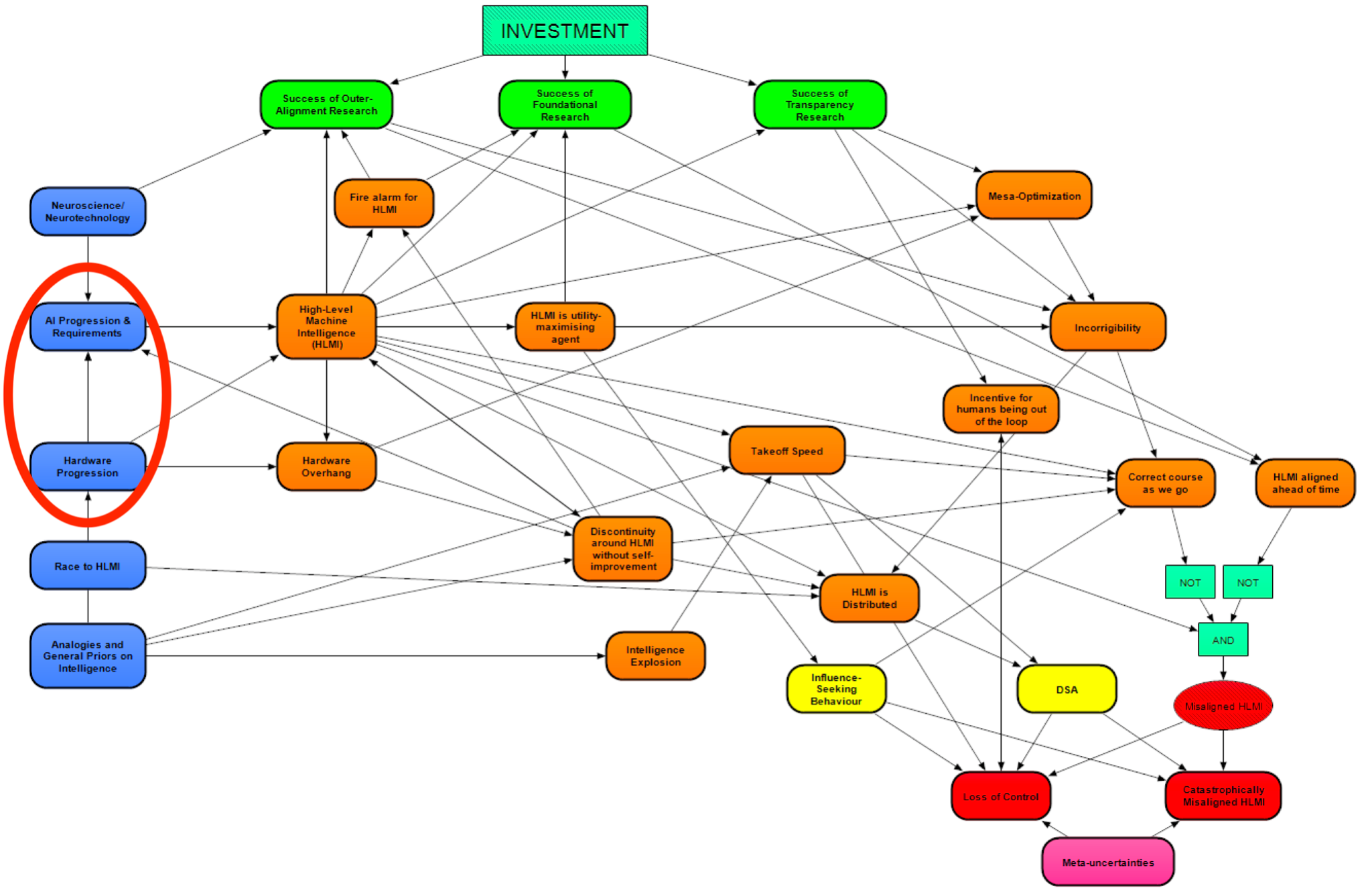
The module AI Progression & Requirements investigates when we should expect HLMI to be developed, as well as what kind of HLMI we should expect (e.g., whole brain emulation [? · GW], HLMI from current deep learning methods, etcetera). These questions about the timing and kind of HLMI are the main outputs from the sections of the model in this post, influencing downstream parts of the model. The timing question, for instance, determines how much time there is for safety agendas to be solved. The question regarding the kind of HLMI, meanwhile, affects many further cruxes, including which safety agendas are likely necessary to solve in order to avoid failure modes, as well as the likelihood of HLMI being distributed versus concentrated.
The module Hardware Progression investigates how much hardware will likely be available for a potential project towards HLMI (as a function of time). This module provides input for the AI Progression & Requirements module. The AI Progression & Requirements module also receives significant input from the Analogies and General Priors on Intelligence module, which was described in the previous post [? · GW] in this sequence.
We will start our examination here with the Hardware Progression module, and then discuss the module for AI Progression & Requirements.
Hardware Progression
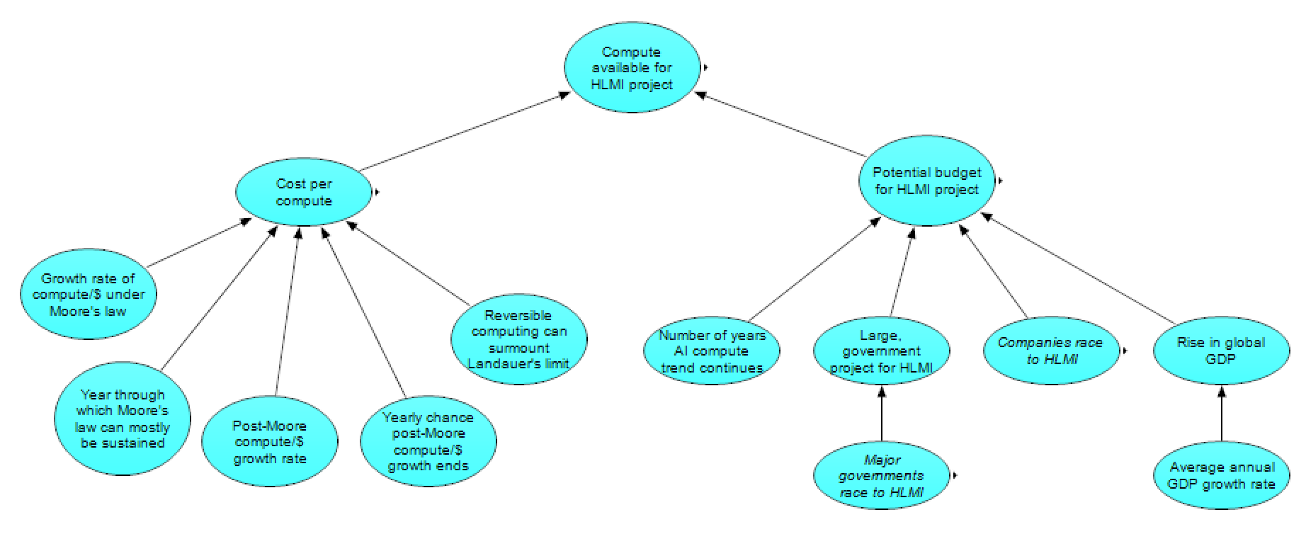
The output from this section is compute available for an HLMI project, which varies by year. This output is determined by dividing the potential budget for an HLMI project by the cost per compute (both as a function of the year).
Cost per Compute
Zooming in on the cost portion, we see the following subgraph:
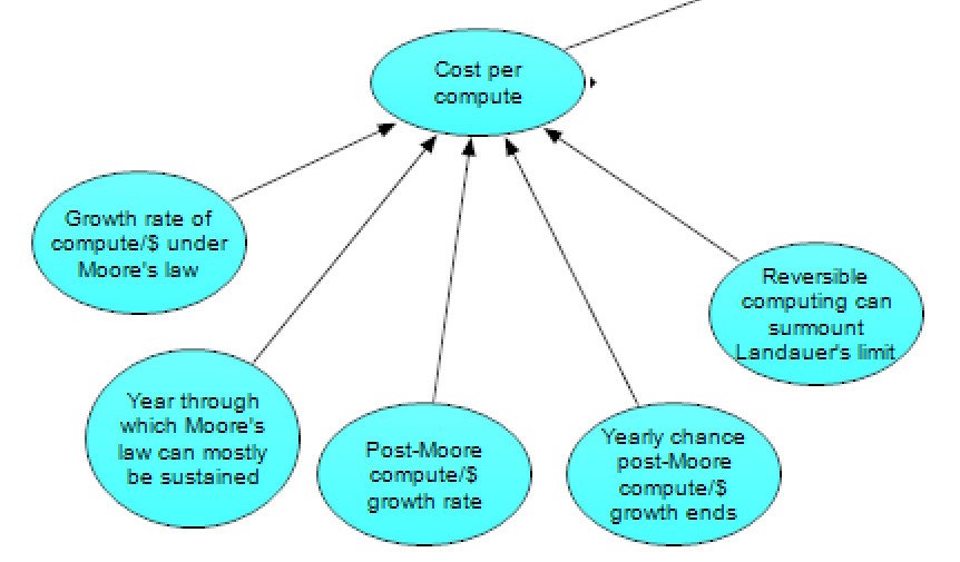
The cost per compute (over time) is the output of this subgraph, and is determined by the other listed nodes. Starting from the current cost of compute, the compute/$ is expected to continue rising until the trend of increasing transistor density on 2D Si chips (i.e., “Moore’s law”) runs out of steam. Note that we’re using “Moore’s law” in the colloquial sense to refer to approximately exponential growth within the 2D Si chip paradigm, not the more specific claim of a 1-2 year doubling time for transistor count. Also note that at this stage, we do not differentiate between CPU, GPU, or ASIC compute, as similar trends apply to all of them. Both the growth rate of compute/$ under the future of Moore’s law and the year through which Moore’s law can mostly be sustained are uncertainties within our model.
After this paradigm ends, compute/$ may increase over time at a new (uncertain) rate (post-Moore compute/$ growth rate). Such a trend could perhaps be sustained by a variety of mechanisms: new hardware paradigm(s) (such as 3D Si chips, optical computing, or spintronics), specialized hardware (leading to more effective compute for the algorithms of interest), a revolution in physical manufacturing (such as via atomically precise manufacturing), or pre-HLMI AI-led hardware improvements. Among technology forecasters, there is large disagreement about the prospects for post-Moore computational growth, with some forecasters predicting Moore-like or faster growth in compute/$ to continue post-Moore, while others expect compute/$ to slow considerably or plateau.
Even if post-Moore growth is initially substantial, however, we would expect compute/$ to eventually run into some limit and plateau (or slow to a crawl), due to either hard technological limits, or economic limits related to increasing R&D and fab costs. The possibility of an eventual leveling off of compute/$ is handled by the model in two different ways. First, there is assumed to be an uncertain, yearly chance post-Moore compute/$ growth ends. Second, Landauer’s limit (the thermodynamic limit relating bit erasure and energy use) may present an upper bound for compute/$, which the model assumes will happen unless reversible computing can surmount Landauer’s limit.
It should be noted that the model does not consider that specialized hardware may present differential effects for different paths to HLMI, nor does it consider how quantum computing might affect progression towards HLMI, nor the possibility of different paradigms post-Moore seeing different compute/$ growth rates. Such effects may be important, but appear complex and difficult to model.
Potential Budget for HLMI Project
The budget section, meanwhile, has this subgraph:
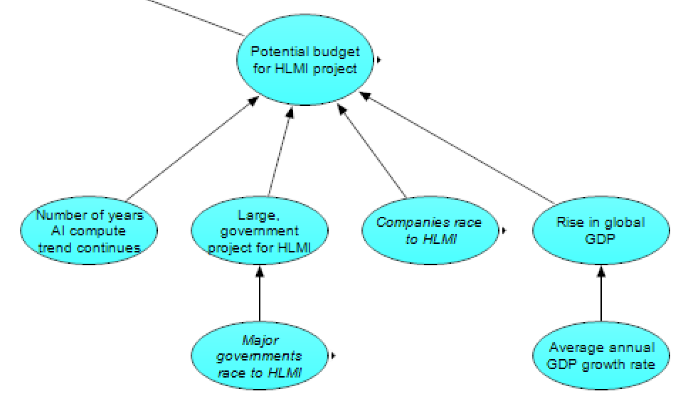
The potential budget for an HLMI project, which is the primary output of this subgraph (used in combination with the output from the previous section on cost per compute to derive the compute available for an HLMI project) is modeled as follows. In 2021, the budget is set to that of the most expensive AI project to date. The recent, quickly-rising AI compute trend may or may not [LW · GW] continue for some number of years, with the modeled budget rising accordingly. After that, the budget for HLMI is currently modeled as generally rising with the rise in global GDP (determined by the average annual GDP growth rate), except if companies race to HLMI (in which case we assume the budget will grow to be similar, in proportion of global GDP, to tech firms’ R&D budgets), or if there’s a large government project for HLMI (in which case we assume budgets will grow to ~1% of the richest country’s GDP, in line with the Apollo program and Manhattan Project). We think such a large government project is particularly likely if major governments race to HLMI.
We should note that our model does not consider the possibility of budgets being cut between now and the realization of HLMI; while we think such a situation is plausible (especially if there are further AI Winters), we expect that such budgets would recover before reaching HLMI, and thus aren’t clearly relevant for the potential budget leading up to HLMI. The possibility of future AI Winters implying longer timelines through routes other than hardware (e.g., if current methods “don’t scale” to HLMI and further paradigm shifts don’t occur for a long time) is, at least implicitly, covered in the module on AI Progression & Requirements.
As our model is acyclic, it doesn’t handle feedback loops well. We think it is worth considering, among other possible feedback loops, how pre-HLMI AI may affect GDP, or how hardware spending and costs may affect each other (such as through economies of scale & learning effects, as well as simple supply and demand), though these effects aren’t currently captured in our model.
AI Progression & Requirements
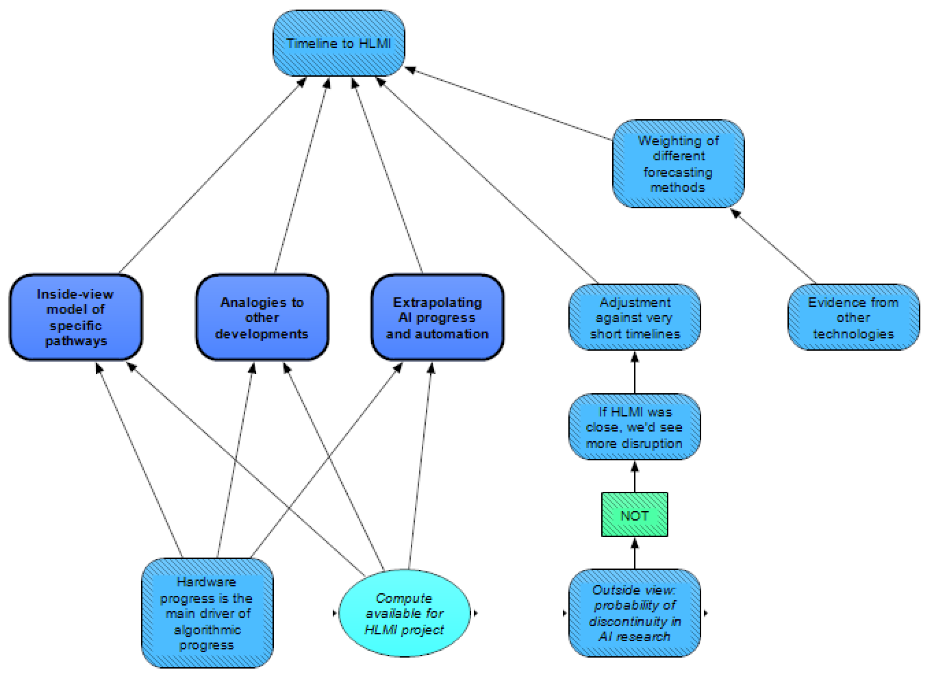
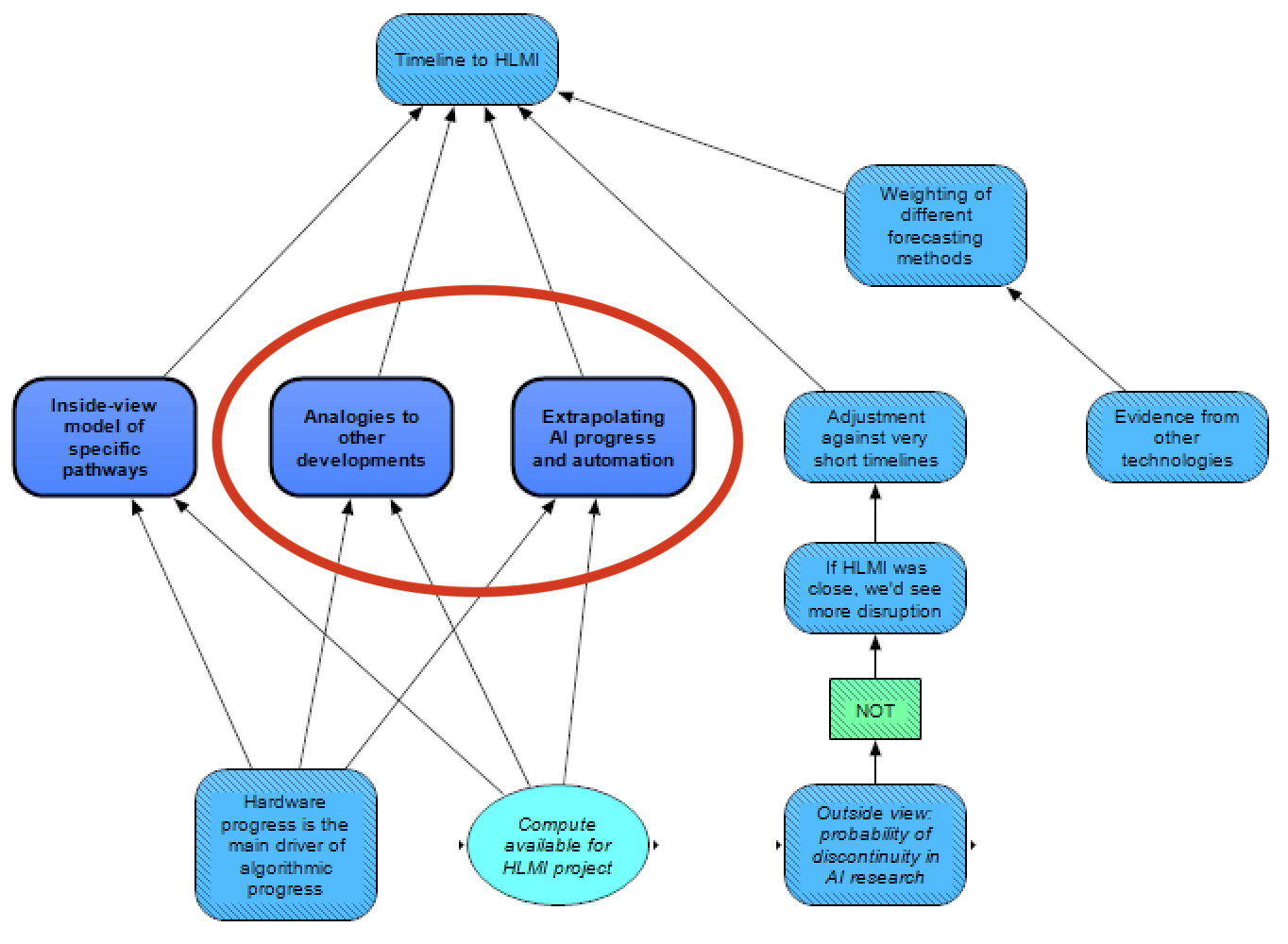
The module on AI Progression & Requirements uses a few different methods for estimating the timeline to HLMI: a gears-level, inside-view model of specific pathways (which considers how various possible pathways to HLMI might succeed), as well as outside-view methods (analogies to other developments, and extrapolating AI progress and automation). All of these methods are influenced by the compute available for an HLMI project (described in the section above), as well as whether or not hardware progress is the main driver of algorithmic progress.
Estimates from these approaches are then combined, currently as a linear combination (weighting of different methods of forecasting timelines), with the weighting based on evidence from other technologies regarding which technological forecasting methods are most appropriate. A (possible) adjustment against very short timelines is also made, depending on whether one believes that if HLMI was close, we’d see more disruption from AI, which in turn is assumed to be less likely if there’s a larger probability of discontinuity in AI research (since such a discontinuity could allow HLMI to “come out of nowhere”).
Inside-view model of specific pathways
This module represents the most intricate of our methods for estimating the arrival of HLMI. Here, several possible approaches to HLMI are modeled separately, and the date for the arrival of HLMI is taken as the earliest date that one of these approaches succeeds. Note that such an approach may introduce an optimizer’s curse [LW · GW] (from the OR gate); if the different pathways have independent errors, then the earliest modeled pathway may be expected to have unusually large error in favor of being early, underestimating the actual timeline. On the other hand, the estimations of the different pathways themselves each contain the combination of different requirements (AND gates), such as requirements for both adequate software and adequate hardware, and this dynamic introduces the opposite bias – the last requirement to fall into place may be expected to have an error in favor of being late. Instead of correcting for these two biases, we simply note that these biases exist in opposite directions, and we are uncertain about which is the larger bias.
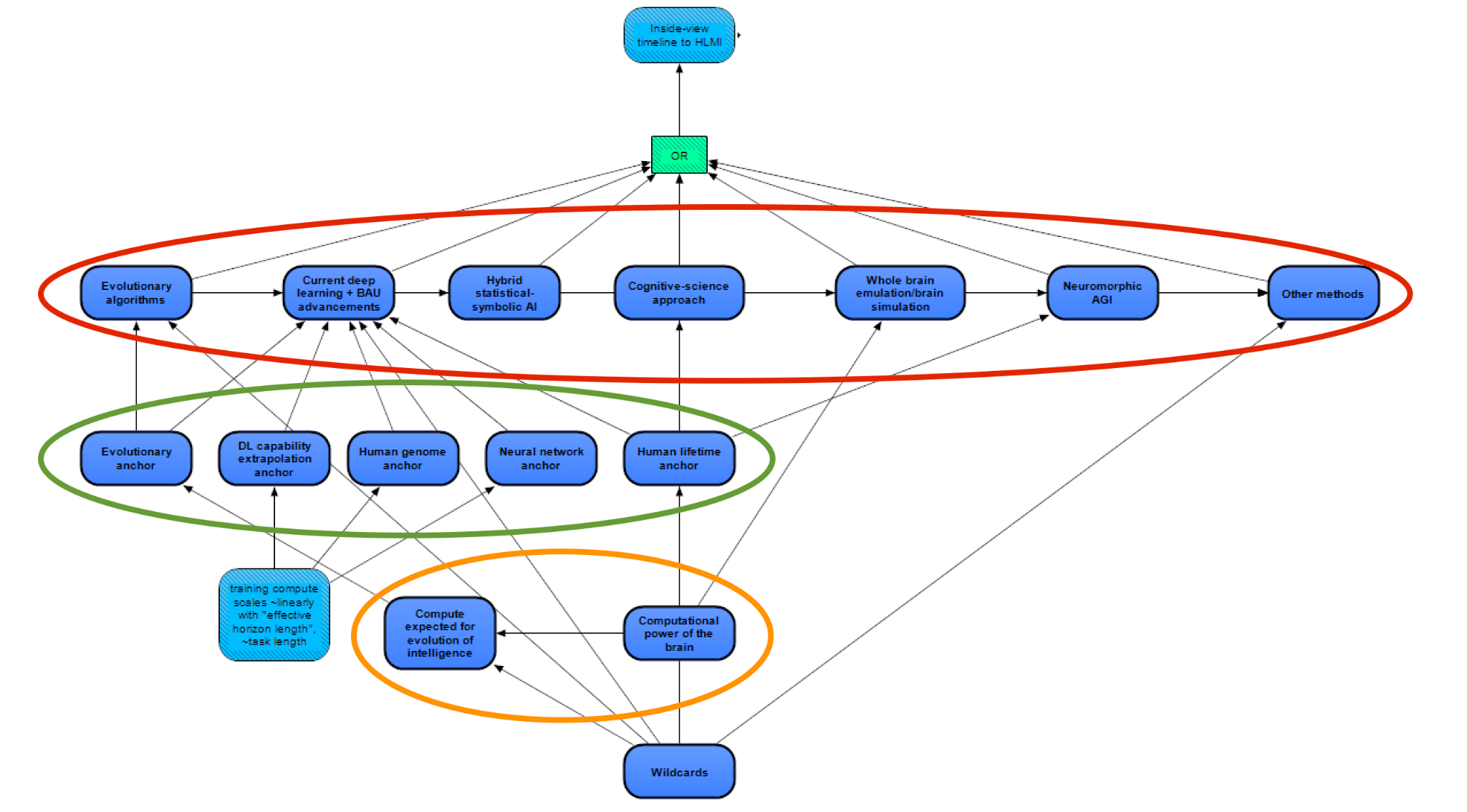
The different methods to HLMI in our model (circled in red above, expanded upon in their individual subsections below) are:
- Evolutionary algorithms – either similar to evolutionary algorithms today, a direct simulation of virtual evolution, or some middle ground. While current evolutionary algorithms are very different from virtual evolution, we have grouped these together instead of grouping current evolutionary algorithms with current deep learning methods, largely because in our model, both of the evolutionary methods rely on similar hardware estimation methods.
- Current deep learning plus business-as-usual advancements – HLMI achieved through methods similar to those in deep learning today; the key features of such methods are large, deep neural nets, trained from a largely “blank-slate” initial state, and optimized via local search techniques such as SGD (though crucially, to avoid double counting, not including evolutionary algorithms).
- Hybrid statistical-symbolic AI – approaches marrying statistical methods and more intentionally designed symbolic methods, such as in GOFAI.
- Cognitive-science approach – approaches to HLMI heavily relying on cognitive science or developmental psychology (likely in combination with deep learning).
- Whole brain emulation / brain simulation – emulating a particular person’s brain in silico (for WBE), or simulating a generic human brain (for brain simulation).
- Neuromorphic AGI – HLMI created using many of the “low-level” processes or architectures of the brain, but without being put together into a virtual brain with particularly humanlike intelligence.
- Other methods – a catch-all, for unanticipated or other potential paths to HLMI.
Each method is generally assumed to be achieved once both the hardware and software requirements are met. The software requirements of the different methods are largely dependent on different considerations, while the hardware requirements are more dependent on different weighting or modifications of the same set of “anchors” (circled in green in the figure above).
These anchors are plausibly-reasonable estimates for the computational difficulty of training an HLMI, based on different analogies or other reasoning that allows for anchoring our estimates. Four of the five anchors come from Ajeya Cotra’s Draft report on AI timelines [AF · GW] (with minor modifications), and we add one more. These five anchors (elaborated upon below) are:
- Evolutionary anchor – an estimate based on the “compute-equivalent” that was “used” in evolution from the first animals with nervous systems to humans (considering both the “brain-compute” used and the compute necessary to simulate the environment sufficiently). This estimate includes both upward and downward adjustments, for possible anthropic effects and for human engineers potentially outcompeting evolution.
- Deep learning capability extrapolation anchor – an estimate of how much compute would be needed to achieve broad, human-level capabilities, given an extrapolation of how capabilities in current deep learning systems scale with compute.
- Human genome anchor – an estimate of the compute needed to train a current ML system sufficiently, based on setting the parameter count to the size of the human genome (arguably the “code” of human intelligence), used in combination with empirically-derived scaling laws and other relevant biological considerations.
- Neural network anchor – an estimate of the compute needed to train a current ML system sufficiently, similar to the human genome anchor, but instead with the parameter count set by considerations related to the compute-equivalent used in the human brain.
- Human lifetime anchor – an estimate of how much compute-equivalent occurs in “training” a human brain from birth to adulthood, increased by a factor for human infants being “pre-trained” by evolution.
Also similar to Cotra, we plan to use lognormal distributions (instead of point estimates) around our anchors for modeling compute requirements, due to uncertainty, spanning orders of magnitude, about these anchors’ “true” values, as well as uncertainty around the anchors’ applicability without modifications. A couple of these anchors are influenced by upstream nodes related to the evolution of intelligence and the computational power of the brain (circled in orange above; these “upstream” nodes are lower down on the figure since the information in the figure flows bottom to top).
Additionally, one final module includes “wildcards” that are particularly speculative but, if true, would be game-changers. The nodes within this wildcards module have been copied over to other relevant modules (to be discussed below) as alias nodes.
We discuss the modules for the various methods to HLMI below, elaborating on the relevant anchors (and more upstream nodes) where relevant.
Evolutionary Algorithms
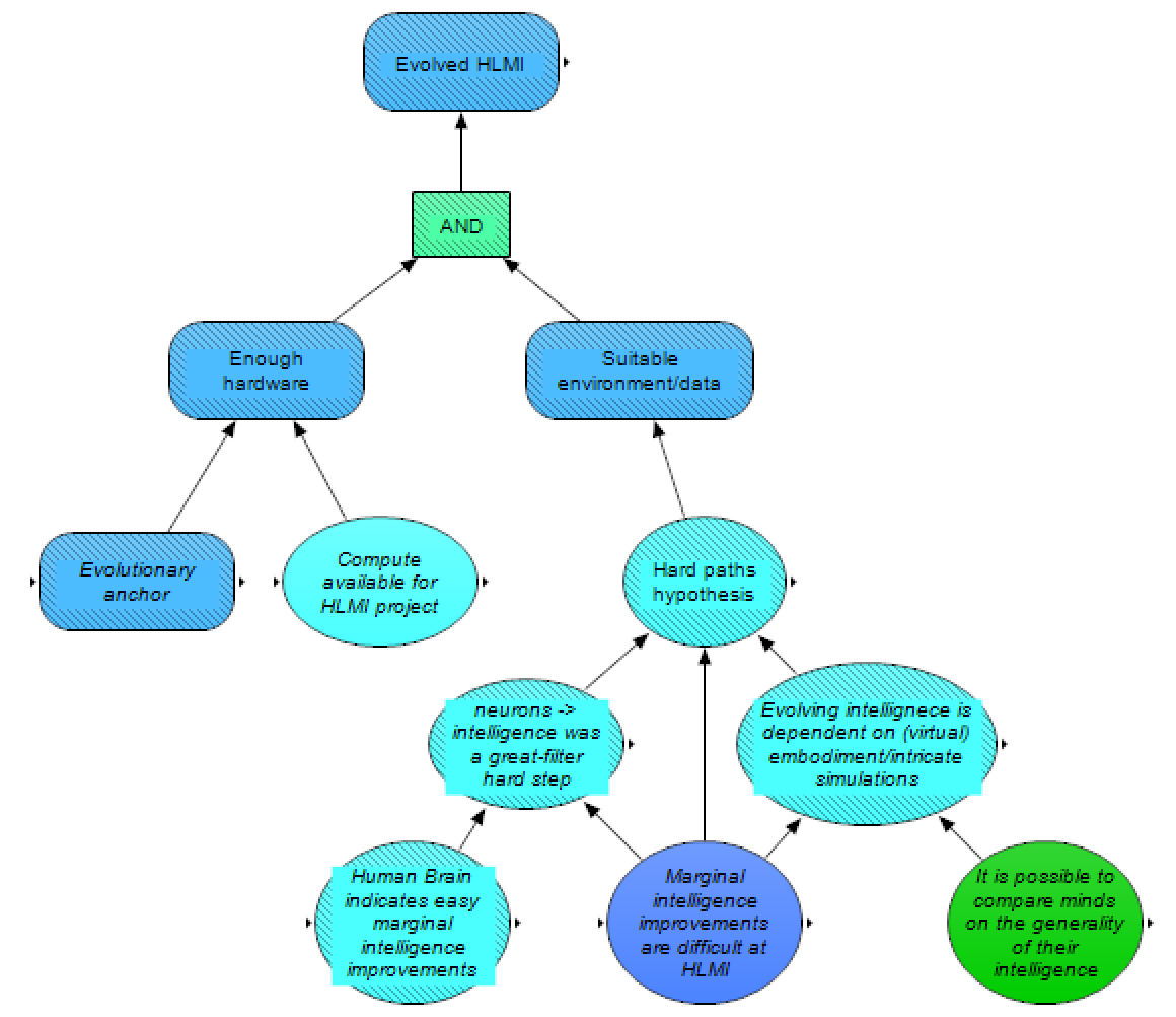
The development of evolved HLMI would require both enough hardware and a suitable environment or other dataset, given the evolutionary algorithm. Whether there will be enough hardware by a specific date depends on both the required hardware (approximated here by the evolutionary anchor, discussed below) and how much hardware is available at that date (calculated in the Hardware Progression module, discussed above). The ability to create a suitable environment/dataset by a certain date depends, in large part, on the hard paths hypothesis [AF · GW] – the hypothesis that it’s rare for environments to straightforwardly select for general intelligence.
This hypothesis is further influenced by other cruxes. If somewhere along the progression from the first neurons to human intelligence, there was a “hard step” (a la the great filter), then such a hypothesis is more likely true. Such a hard step would imply that the vast majority of planets that evolve animal-like life with neuron-like parts never go on to evolve a technologically intelligent lifeform. This scenario could be the case if Earth (or some portion of Earth’s history) was particularly unusual in some environmental factors that selected for intelligence. Due to anthropic effects, we cannot rule out such a hard step simply based on the existence of (human) technological intelligence on Earth. Such a hard step is less likely to be the case if marginal intelligence improvements are easy around the human level, and we consider evidence from the human brain (such as whether the human brain appears to be a “scaled up” version of a more generic mammalian or primate brain) to be particularly informative here (both of these cruxes are copied over from our module on Analogies and General Priors on Intelligence, described in the previous post [AF · GW]).
Additionally, the hard paths hypothesis is influenced by whether evolving intelligence would depend on embodiment (e.g., in a virtual body and environment). Proponents of this idea have argued that gaining sufficient understanding of the physical world (and/or developing cognitive modules for such understanding), including adequate symbol grounding [AF · GW] of important aspects of the world and (possibly necessary) intuitive physical reasoning (e.g., that humans use for certain mathematical and engineering insights), would require an agent to be situated in the world (or in a sufficiently realistic simulation), such that the agent can interact with the world (or simulation). Opponents of such claims often argue that multi-modal learning will lead to such capabilities, without the need for embodiment. Some proponents further claim that even if embodiment is not in principle necessary for evolving intelligence, it may still be necessary in practice, if other environments tend to lack the complexity or other attributes that sufficiently select for intelligence.
If evolving intelligence depends on embodiment, this would significantly decrease the potential paths to evolving intelligence, as HLMI would therefore only be able to be evolved in environments in which it was embodied, and also potentially only in select simulated environments that possessed key features. The necessity of embodiment appears to be less likely if marginal intelligence improvements are easy. In particular, the necessity of embodiment appears less likely if minds can be compared on the generality of their intelligence (also copied over from our module on Analogies and General Priors on Intelligence [AF · GW]), as the alternative implies “general intelligence” isn’t a coherent concept, and intelligence is then likely best thought of as existing only with respect to specific tasks or goals; in such a situation, AI systems interacting in or reasoning about the physical world would likely need to have the development of their cognitive faculties strongly guided by interactions in such a world (or a close replica).
Finally, even if there is no evolutionary hard step between neurons and intelligence and embodiment is not necessary for evolving intelligence, the hard paths hypothesis may still be true; some have argued [AF · GW], for example, that curriculum learning may be necessary for achieving HLMI. It therefore seems reasonable to assume that the harder marginal intelligence improvements are around the HLMI level (even holding constant the other mentioned cruxes), the lower chance we should give to an individual environment/dataset leading to the evolution of intelligence, and thus the higher credence we give the hard paths hypothesis.
As mentioned above, on the compute side, the requirements for evolved HLMI are dependent on the evolutionary anchor. This anchor is determined by an upstream submodule (the Evolutionary anchor submodule). Our estimate for this anchor is similar to its analog in Cotra’s report [AF · GW], but with a couple of key differences:
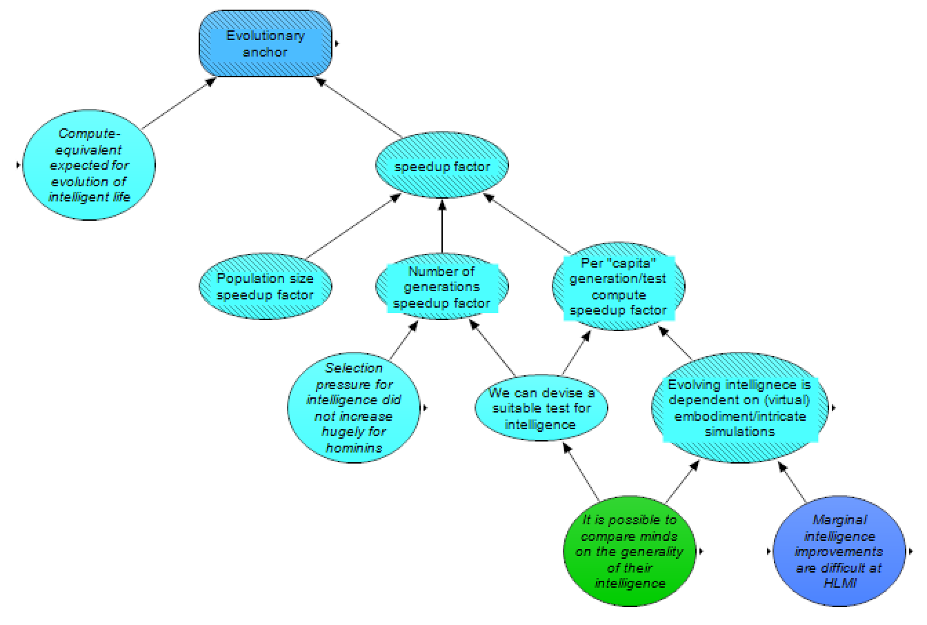
Here, this anchor is determined by taking the amount of “compute-equivalent” expected for the evolution of intelligent life such as humans (considering both neural activity and simulating an environment), and dividing it by a speedup factor due to human engineers potentially being able to outcompete biological evolution towards this goal. Cotra’s report did not include such a speedup factor, as she was using her evolutionary anchor as somewhat of an upper bound. Here, on the other hand, we are instead concerned with an all-things-considered estimate of how difficult it would be to evolve HLMI.
Our speedup factor considers three sources of increased speed:
- Population size speedup factor – the population of Earth’s animals is not set by minimizing the amount of compute-equivalent necessary to evolve an intelligent species, but instead by Earth’s carrying capacity; human engineers, meanwhile, could set population sizes with the goal of minimizing necessary compute to evolve intelligence.
- Number of generations speedup factor – much of Earth’s macroevolutionary history was presumably not optimizing for an intelligent species in as few generations as possible, and there are many tricks that human engineers could employ to select for and possibly achieve this goal quicker. In particular, if evolution was hardly selecting for intelligence before hominins, then a more intentional effort could likely be much faster. Additionally, if we can design tests for intelligence, then we could potentially create stronger selection pressure for intelligence, reducing the simulated time needed.
- Per “capita” speedup factor – for biological evolution, organisms are “run” from birth until they die, despite much of that time not necessarily presenting much selection effect. Human engineers might be more efficient here – especially if we can devise a test for intelligence (in which case the generation time might be whatever is required to complete a short test) and/or if evolving intelligence does not depend on embodiment (in which case much of the information processes in animals’ brains is likely, in principle, unimportant for evolving intelligence, and thus human engineers could reduce compute requirements by crafting much simpler datasets that don’t lead to costly adaptations for embodiment).
Note that there is somewhat of a tradeoff between these three factors – a smaller population, for instance, would presumably imply more generations needed. Each of these factors should therefore be set to minimize the product of the three variables instead of only the corresponding variable itself.
The expected amount of compute-equivalent required to evolve intelligence on Earth (not considering the speedup factor – i.e., the left node in the above diagram) is estimated from a further upstream submodule, compute expected for evolution of intelligence, which is represented below.
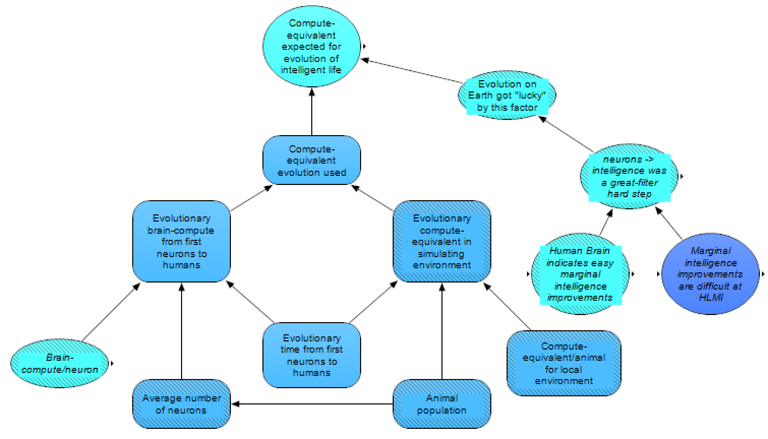
This estimate is made up of two main factors which are multiplied together: the compute-equivalent evolution used on Earth, and a factor related to the possibility that evolution on Earth got “lucky”. The latter of these factors corresponds to the aforementioned possibility that there was a hard step between the first neurons and humans – this factor is set to 1 if either there was no hard step or if there was a hard step relating strictly to Earth’s environment being unusual, and otherwise the factor is set to a number higher than one, corresponding to how much faster evolution of intelligence (from first neurons) took compared to, naively, how long such a process would be expected to take given an Earth-like environment and infinite time. That is, the factor is more-or-less set to an estimate to the question, “For every Earth-like planet that evolves a lifeform with technological intelligence, how many Earth-like planets evolve a lifeform with something like Precambrian jellyfish intelligence?”
The factor for compute-equivalent evolution used, meanwhile, is broken up into the sum of two factors: the brain-compute from first neurons to humans (i.e., based on an estimate of how much compute each nervous system “performs”, though note the definition here is somewhat inexact) and the compute-equivalent used in simulating the environment (i.e., an estimate of the minimum compute necessary to simulate an environment for the evolution of animals on Earth). The environmental compute-equivalent factor has traditionally been neglected in analyzing the compute-equivalent for simulating evolution, as previous research has assumed that much more necessary compute occurs in brains than in the surrounding environment (for instance, because the human brain uses much more brain-compute than the compute in even high-resolution video games, and humans can function in such environments, including interacting with each other). While this assumption may be reasonable for the functioning of large animals such as humans, it is not immediately obvious that it also applies to much smaller animals such as C. elegans. Furthermore, environmental complexity, dynamism, and a large action-space are typically thought to be important for the evolution of intelligence, and a more complex and dynamic environment, especially in which actors are free to take a very broad set of actions, may be more computationally expensive to simulate.
Both the brain-compute estimate and the environmental compute-equivalent estimate are determined by multiplying the evolutionary time from first neurons to humans by their respective populations, and then by the compute-equivalent per time of each member within these populations. For the brain-compute estimate, the population of interest is the neurons, so the relevant factors are average number of neurons (in the world) and the brain-compute per neuron (as has been estimated by Joseph Carlsmith). For the environmental compute-equivalent estimate, the relevant factors are the average population of animals (of course, related to the average population of neurons), and the compute required to simulate the local environment for the average animal (under the idea that the local environment surrounding animals may have to be simulated in substantially higher resolution than parts of the global environment which no animal occupies).
To recap, adding together the brain-compute estimate and the environmental compute-equivalent estimate yields the total estimate for compute-equivalent evolution used on Earth, and this estimate is then multiplied by the “luckiness” factor for the compute-equivalent expected to be necessary for evolving intelligence. The evolutionary anchor is then determined by multiplying this factor by a speedup factor. The date by which enough hardware is available for evolved HLMI is set to be the first date the available compute for an HLMI project exceeds the evolutionary anchor, and evolved HLMI is assumed to be created on the first date that there is enough hardware and a suitable environment or dataset (which is strongly influenced by the hard paths hypothesis).
Current Deep Learning plus Business-As-Usual Advancements
This module, which represents approaches towards HLMI similar to most current approaches used in deep learning, is more intricate than the others, though also relies on some similar cruxes to the above.
Similar to evolutionary algorithms, we model achieving this milestone at the first date that there is both enough hardware (given the available algorithms) and sufficient data (quantity, quality, and kind, again given the available algorithms) for training the HLMI.
The ease of achieving the necessary data is strongly influenced by the hard paths hypothesis [AF · GW] (circled in red above), as before.
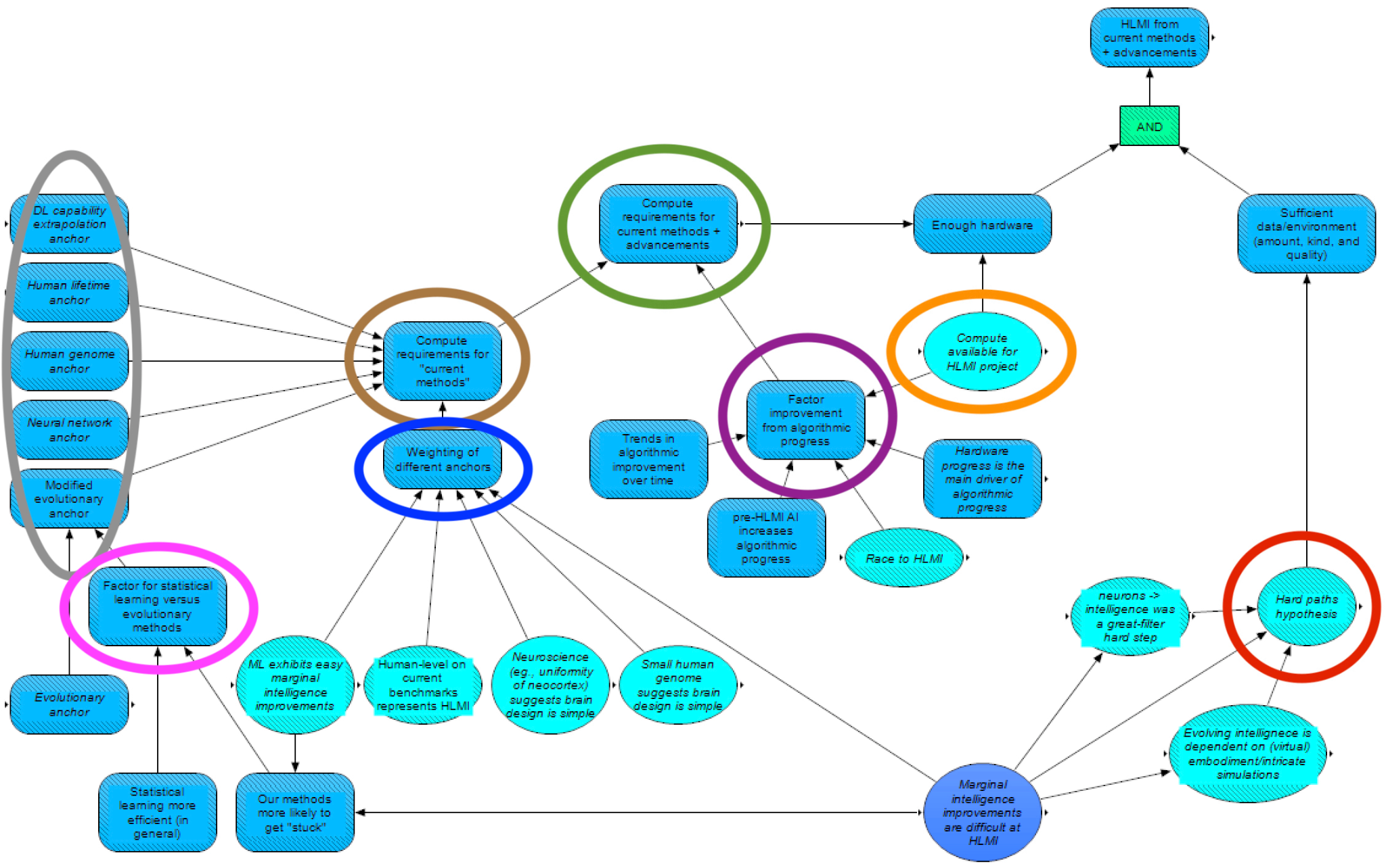
Whether enough hardware will exist for HLMI via these methods (by a certain date) is determined by both the amount of hardware available (circled in orange) and the hardware requirements (circled in green). As before, the hardware available is taken from the Hardware Progression module. The hardware requirements, in turn, are determined by the compute requirements for “current methods” in deep learning to reach HLMI (circled in brown), modified by a factor for algorithmic progress (circled in purple). Expected algorithmic improvements are modeled as follows.
First, baseline algorithmic improvements are extrapolated from trends in such improvements. This extrapolation is performed, by default, in terms of time. However, if the crux hardware progress is the main driver of algorithmic progress resolves positively, then the extrapolation is instead based on hardware progress, proxied with compute available for an HLMI project. Next, the baseline algorithmic improvements are increased if there is a race to HLMI (in which case it is assumed investment into algorithmic advancements will increase), or if it is assumed that pre-HLMI AI will enable faster AI algorithmic progress.
Compute requirements for “current methods” are estimated as a linear combination of the estimates provided by the anchors (circled in grey). The evolutionary anchor is modified by a factor (circled in pink) for whether our statistical learning algorithms would be better/worse than the evolutionary anchor in terms of finding intelligence. The main argument in favor of our statistical methods is that statistical learning is generally more efficient than evolution, and the main argument against is that our statistical methods may be more likely to get “stuck” [AF · GW], either via strongly separated local minima, or due to goal hacking and Goodhart’s Law becoming dead-ends for sufficiently general intelligence (which may be less likely if marginal improvements in intelligence near HLMI are easier, and particularly less likely if ML shows evidence of easy marginal intelligence gains).
Our estimates for the human lifetime anchor, human genome anchor, and neural network anchor are all calculated using the similar logic as in Cotra’s report [AF · GW]. The human lifetime anchor involves estimating the brain-compute that a human brain performs in “training” from birth to adulthood – i.e., (86 billion neurons in a human brain)*(brain-compute per neuron per year)*(18 years) – and multiplying this number by a factor for newborns being “pre-trained” by evolution. This pre-training factor could be based on the extent to which ML systems today are “slower-learners” compared to humans, or the extent to which human-engineered artifacts tend to be less efficient than natural analogs.
The human genome anchor and neural network anchor, meanwhile, are calculated in somewhat similar manners to each other. In both, the modeled amount of compute to train an HLMI can be broken down into the amount of data to train the system, times the compute used in training per amount of data. The number of data points needed can be estimated from the number of parameters the AI uses, via empirically-derived scaling laws between parameters and data points for training, with the number of parameters calculated differently for the different anchors: for the human genome anchor, it’s set to the bytes in the human genome, and for the neural network anchor, it’s set based on expectations from scaling up current neural networks to use similar compute as the brain (with a modifying factor). The compute used in training per data point for both of these anchors, meanwhile, is calculated as the brain-compute in the human brain, time a modifying factor for the relative efficiency of human engineered artefacts versus their natural analogs, times the amount of “subjective time” generally necessary to determine if a model perturbation improves or worsens performance (where “subjective time” is set from the amount of compute the AI uses, such that the compute the AI uses equals the brain-compute the human brain uses, times the modifying factor, times the subjective time). For this last factor regarding the subjective time for determining if a model perturbation is beneficial or harmful (called the “effective horizon length”), for the human genome anchor, the appropriate value is arguably related to animal generation times, while for the neural network anchor, the appropriate value is arguably more related to the amount of time that it takes humans to receive environmental feedback for their actions (i.e., perhaps seconds to years, though for meta-learning or other abilities evolution selected for, effective horizon lengths on par with human generation times may be more appropriate). For a more in-depth explanation of the calculations related to these anchors, see Cotra’s report [AF · GW] or Rohin Shah’s summary of the report.
Finally, our model includes an anchor for extrapolating the cutting edge of current deep learning algorithms (e.g., GPT-3 [AF · GW]) along various benchmarks in terms of compute – effectively, this anchor assumes that deep learning will (at least with the right data) “spontaneously” overcome its current hurdles (such as building causal world models, understanding compositionality, and performing abstract, symbolic reasoning) in such a way that progress along these benchmarks will continue their current trends in capabilities vs compute as these hurdles are overcome.
The human genome anchor, neural network anchor, and DL capability extrapolation anchor all rely on the concept of the effective horizon length, which potentially provides a relationship between task lengths and training compute. Resultantly, disagreements related to these relationships are cruxy. One view is that, all else equal, effective horizon length is generally similar to task length, and training compute scales linearly with effective horizon length. If this is not the case, however, and either effective horizon length grows sublinearly with task length, or training scales sublinearly with effective horizon length, then all three of these anchors could be substantially shorter. While our model currently has a node for whether training time scales approximately linearly with effective horizon length and task length, we are currently uncertain how to model these relationships if this crux resolves negative. An intuition pump in favor of sublinearity between training time and task length is that if one has developed the qualitative capabilities necessary to write a 10-page book, one also likely has the qualitative capabilities necessary to write a 1,000-page book; writing a 1,000-page book might itself take 100 times as long as writing a 10-page book, but training to write a 1,000-page book presumably does not require 100 times longer than training to write a 10-page book.
The weighting of these five anchors (circled in blue) is also a subject of dispute. We model greater weighting towards lower anchors if marginal intelligence improvements around HLMI are easy, and we additionally weight several of the specific anchors higher or lower depending on other cruxes. Most importantly, the weighting of the DL capability extrapolation anchor is strongly dependent on whether human-level on current benchmarks represents HLMI and if ML exhibits easy marginal intelligence improvements (implying such extrapolations are more likely to hold until humal level, as compute is ramped up). The human lifetime anchor is weighted higher if neuroscience suggests the brain design is simple (since then, presumably, the human mind is not heavily fine-tuned due to pretraining). Additionally, if the small human genome suggests that the brain design is simple, then the human genome anchor is weighted higher (otherwise, we may assume that the complexity of the brain is higher than we might assume from the size of the genome, in which case this anchor doesn’t make a lot of sense).
Let’s consider how a couple of archetypal views about current methods in deep learning can be represented in this model. If one believes that DL will reach HLMI soon after matching the compute in the human brain (for instance, due to the view [AF · GW] that we could make up for a lack of fine-tuning from evolution with somewhat larger scale), then this would correspond to high weight on the human lifetime anchor, in combination with a “no” resolution for the hard paths hypothesis. On the other end of the spectrum, if one were to believe that “current approaches in DL can’t scale to HLMI”, then this would presumably correspond to either a sufficiently strong “yes” to the hard paths hypothesis (that is, “current methods could scale if we had the right environment or data, but such data will not be created/aggregated, and the wrong kind of data won’t lead to HLMI”), or a high weight to the modified evolutionary anchor, with, presumably, either a very large factor for our methods getting “stuck” (“evolution was only able to find intelligence due to evolution having advantages over our algorithms”), or a large factor for “luckiness” of evolution (“evolution got astronomically lucky to reach human-level intelligence, and even with evolutionary amounts of compute, we’d still be astronomically unlikely to reach HLMI”).
Hybrid statistical-symbolic AI
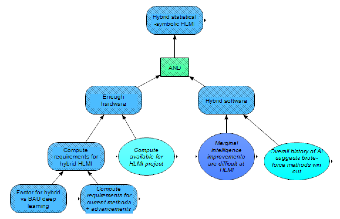
Many people who are doubtful about the ability of current statistical methods to reach HLMI instead think that a hybrid statistical-symbolic approach (e.g., DL + GOFAI) could be more fruitful. Such an approach would involve achieving the necessary hardware (similar to before) and creating the necessary symbolic methods, data, and other aspects of the software. Here, we model the required hardware as being related to the required hardware for current deep learning + BAU (business-as-usual) advancements (described in the above section), modified with a factor for hybrid methods requiring more/less compute. As we are not sure how best to model achieving the necessary software (we are open to relevant suggestions), our model of this is very simple – we assume that such software is probably easier to develop if marginal intelligence improvements are easier, and further that the stronger one buys the bitter lesson, that there is a history of more naive, compute-leveraging, brute-force methods winning compared to more manually crafted methods, the less one should suspect such hybrid software is feasible.
Cognitive-science approach
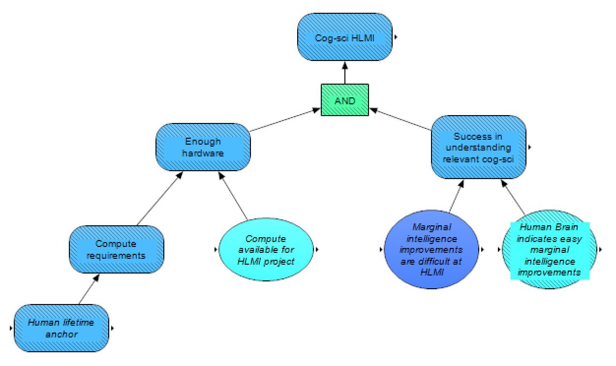
Similar to the above section, some people who are doubtful about the prospects of deep learning have suggested insights from cognitive science and developmental psychology would enable researchers to achieve HLMI. Again, this approach requires the relevant hardware and software (where the software is now dependent on understanding the relevant cognitive science). The hardware requirement here is estimated via the human lifetime anchor, as the cognitive science approach is attempting to imitate the learning processes of the human mind more closely. Again here, we are unsure how to model the likelihood in software success (ideas for approaching this question would be appreciated). For the time being, we assume that, similar to with other methods, the easier marginal intelligence is, the more likely this method will work, and in particular evidence from the brain would be particularly informative here, as a simpler human brain would presumably imply an easier time copying certain key features of the human mind.
Whole brain emulation/brain simulation
These methods would involve running a model of a brain (in the case of WBE, of a specific person’s brain, and in the case of brain simulation, of a generic brain) on a computer, by modeling the structure of the brain and the information-processing dynamics of the lower-level parts of the brain, as well as integrating this model with a body inside an environment (either a virtual body and environment, or a robotic body with I/O to the physical world). To be considered successful for our purposes here, the model would have to behave humanlike (fulfilling the criteria for HLMI), but (in the case of WBE) would not need to act indistinguishable from the specific individual whose brain was being emulated, nor would it have to accurately predict the individual’s behavior. We can imagine, by analogy to weather forecasting, that accurately forecasting the weather is much harder than simply forecasting weather-like behavior, and similarly the task outlined here is likely far easier than creating a WBE with complete fidelity to an individual’s behavior, especially given the potential for chaos.
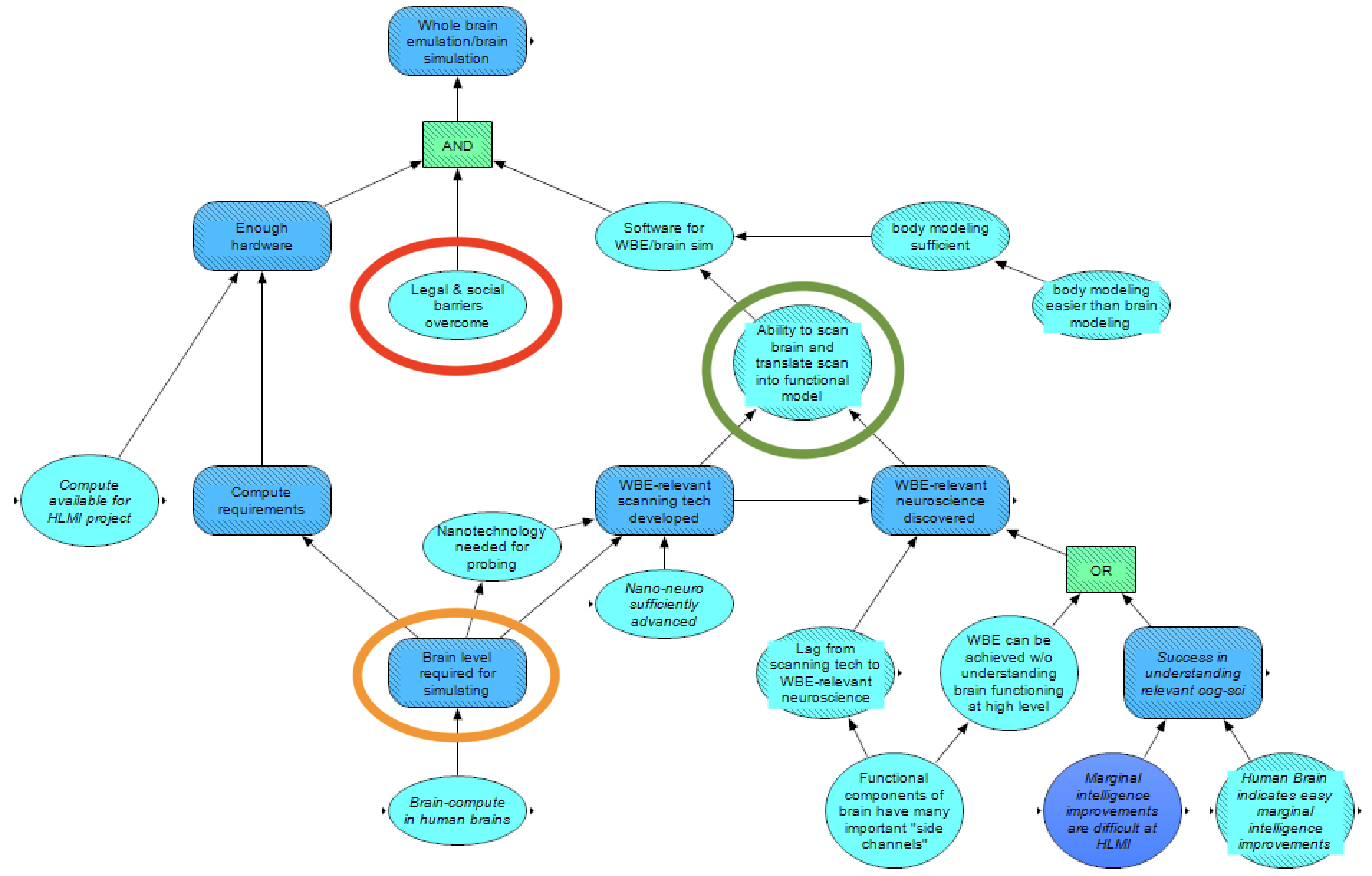
As before, our Analytica model considers cruxes for fulfilling hardware and software requirements, but we also include a node here for overcoming the legal and social barriers (circled in red). This is due to the fact that many people find the idea of brain emulation/simulation either ethically fraught or intuitively disturbing and unpalatable, and it is therefore less likely to be funded and pursued, even if technologically feasible.
As before, the hardware question is determined by availability and requirements, with requirements dependent on the scale at which the brain must be simulated (e.g., spiking neural network, concentrations of neurotransmitters in compartments, and so on) – circled in orange. We consider that the more brain-compute that the human brain uses (number of neurons times brain-compute per neuron), the lower scale we should assume must be simulated, as important information processing is then presumably occurring in the brain at lower scales (interactions on lower scales tend to be faster and larger in absolute number); however, the amount of brain-compute the brain uses is modeled here as a lower bound on computational costs, as emulating/simulating might require modeling details less efficiently than how the brain instantiates its compute (in the same way that a naive simulation of a calculator – simulating the electronic behavior in the various transistors and other electronic parts – would be much more computationally expensive than simply using the calculator itself).
On the software side, success would be dependent on the ability to scan a brain and translate the scan into a functional model (circled in green) and to model a body sufficiently (with one potential crux for whether body modeling is easier than brain modeling). Scanning the brain sufficiently, in turn, is dependent on WBE-relevant scanning technology enabling the creation of a structural model of the brain (at whatever scale is necessary to model), while translating the scan into a model would depend on the discovery of WBE-relevant neuroscience that allows for describing the information-processing dynamics of the parts of the brain. Note that, depending on the scale necessary to consider for the model, such “neuroscience” might include understanding of significantly lower-level behavior than what’s typically studied in neuroscience today.
Discovering the relevant neuroscience, in turn, would depend on a few factors. First, relevant scanning technology would need to be created, so that the dynamics of the brain could be probed adequately. Such scanning technology would presumably include some similar scanning technology as mentioned above for creating a structural model, though would also likely go beyond this (our model collapses these different types of scanning technology down to one node representing all the necessary scanning technology being created). Second, after such scanning technology was created, there would plausibly be a lag from the scanning technology to the neuroscience, as somewhat slow, physical research would presumably need to be carried out with the scanning technology to discover the relevant neuroscience.
Third, neuroscientific success would depend on either brain emulation/simulation being achievable without understanding the brain functioning at a high level, or there would need to be success in understanding sufficient cognitive science (which we proxy with the same understanding necessary for a cognitive-science HLMI). Such higher-level understanding may be necessary for validating the proper functioning of components on various scales (e.g., brain regions, large-scale brain networks, etcetera) before integrating them.
We plan to model both the length of the lag and whether WBE can be achieved without understanding the higher-level functioning of the brain as dependent on whether there are many important “side channels” for the I/O behavior of the functional components of the brain. If there are many such side channels, then we expect finding all of them and understanding them sufficiently would likely take a long time, increasing the lag considerably. Furthermore, validating the proper functioning of parts in this scenario would likely require reference to proper higher-level functioning of the brain, as the relevant neural behavior would resultantly be incredibly messy. On the other hand, if there are not many such side channels, discovering the proper behavior of the functional parts may be relatively quick after the relevant tools for probing are invented, and appropriate higher-level functioning may emerge spontaneously from putting simulated parts together in the right way. Arguments in favor [AF · GW] of there being many side channels typically make the point that the brain was biologically evolved, not designed, and evolution will tend to exploit whatever tools it has at its disposal in a messy way, without heed to legibility. Arguments against there being many such side channels typically take the form that the brain is fundamentally an information-processing machine, and therefore its functional parts, as signal processors, should face strong selection pressure for maintaining reliable relationships between inputs and outputs – implying relatively legible and clean information-processing behavior of parts.
Developing the necessary scanning technology for WBE, meanwhile, also depends on a few factors. The difficulty of developing the technology would depend on the brain level required to model (mentioned above). Additionally, if the scanning technology requires nanotechnology (likely dependent on the brain level required for simulating), then an important crux here is whether sufficient nano-neurotechnology is developed.
Neuromorphic AGI (NAGI)
To avoid one point of confusion between this section and the two previous sections: the previous section (WBE/brain simulation) is based on the idea of creating a virtual brain that operates similar to a biological brain, and the section before that (cognitive-science approach) is based on the idea of creating HLMI that uses many of the higher-level processes of the human mind, but that isn’t instantiated on a lower-level in a similar manner to a biological brain (e.g., such an approach might have modules that perform similar functions to brain regions, but without anything modeling bio-realistic neurons). In contrast, this section (neuromorphic AGI) discusses achieving HLMI via methods that use lower-level processes from the brain, but without putting them together in a manner to create something particularly human mind-like (e.g., it may use models of bio-realistic neurons, but in ways at least somewhat dissimilar to human brain structures).
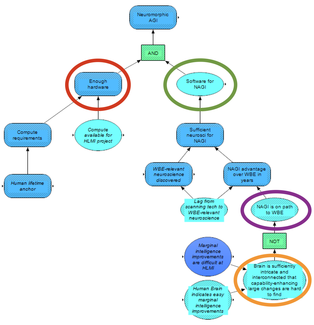
Similar to other methods, NAGI is modeled as being achieved if the relevant hardware (circled in red) and software (circled in green) are achieved. As with the cognitive-science approach, the human lifetime anchor is used for the compute requirement (which is compared against the available compute for whether there is enough hardware), as this method is attempting to imitate more humanlike learning.
On the software side, the main crux is whether NAGI is on the path to WBE (circled in purple). If so, then the relevant neuroscience for NAGI (sufficient for the software for NAGI) is assumed to be discovered before the relevant neuroscience for WBE. The amount of time advantage that NAGI has over WBE in terms of relevant neuroscience under this condition is then assumed to be less than or equal to the lag from scanning technology to WBE-relevant neuroscience; that is, the neurotechnology needed for NAGI is implicitly assumed to be the same as for WBE, but gathering the relevant neuroscience for NAGI is assumed to be somewhat quicker.
Whether NAGI is on the path to WBE, however, is dependent on whether the brain is sufficiently intricate and interconnected that large changes are almost guaranteed to worsen capabilities (circled in orange; if so, then NAGI is assumed to not be on the path to WBE, because potential “modifications” of brain architecture to create NAGI would almost definitely hurt capabilities). This crux is further influenced by the difficulty of marginal intelligence improvements, with particular emphasis on evidence from the human brain.
Other Methods
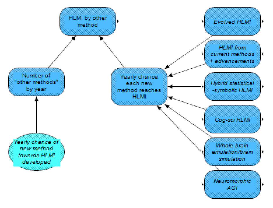
As a catch-all for other possible methods, we have a section for other methods, which depends on the yearly chance of new methods being developed and the yearly chance each of these new methods reaches HLMI.
As both of these uncertainties are deeply unknown, we plan on taking a naive, outside-view approach here. (We are open to alternative suggestions or improvements.) The field of AI arguably goes back to 1956, and over these 65 years, we now arguably have around six proposed methods for how to plausibly get to HLMI (i.e., the other six methods listed here). Other characterizations of the different paths may yield a different number, for example by combining the first two methods into one, or breaking them up into a few more, but we expect most other characterizations would not tend to differ from ours drastically so – presumably generally within a factor of 2. Taking the assumption of six methods developed within 65 years at face value, this indicates a yearly chance of developing a new method towards HLMI of ~9%. (Though we note this assumption implies the chances of developing a new method is independent each year to the next, and this assumption is questionable.) For the second uncertainty (the chance the methods each reach HLMI in a year), the relationship is also unclear. One possible approach is to simply take the average chance of all the other methods (possibly with a delay of ~20 years for the method to “scale up”), but this will likely be informed by further discussion and elicitation.
Outside-view approaches
In addition to the inside-view estimation for HLMI timelines based on specific pathways, we also estimate HLMI arrival via outside-view methods – analogies to other developments and extrapolating AI progress and automation.
Analogies to other developments
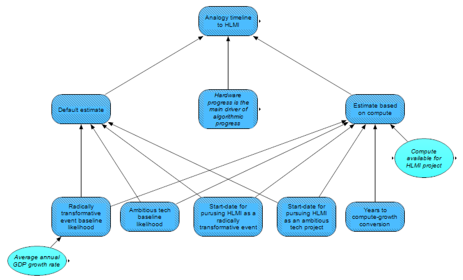
For this module, we take an approach similar to Tom Davidson’s in his Report on Semi-informative Priors, though with some simplifications and a few different modeling judgements.
First, the likelihood of HLMI being developed in a given year is estimated by analogizing HLMI to other classes of developments. This initial, baseline likelihood is estimated in a very naive manner – blind to the history of AI, including to the fact that HLMI has not yet been developed, and instead only considering the base rate for “success” in these reference classes. The two classes of events we use (in agreement with Davidson’s two preferred classes) are: highly ambitious but presumably physically possible projects seriously pursued by the STEM community (e.g., harnessing nuclear energy, curing cancer, creating the internet), and radically transformative events for human work and all of human civilization (the only examples in this reference class are the Agricultural Revolution and the Industrial Revolution).
For both of these reference classes, different methods can be used to estimate the baseline yearly likelihood of “success”; here, we sketch out our current plans for making such estimates. For the ambitious-STEM-projects class, the baseline yearly likelihood can be estimated as simply taking the number of successes for such projects (e.g., 2 for the above three listed ones, as nuclear energy and the internet were successful, while a cure from cancer has not been successful yet) and dividing this number by the sum of the number of years that each project was seriously pursued by the STEM community (e.g., around 5-10 years for pursuing nuclear energy, plus around 50 years for pursuing a cure for cancer, plus perhaps 30 years for the development of the internet, implying, if these three were a representative list, a baseline yearly likelihood of around (2 successes)/(8 + 50 + 30 years) = ~2.3%). Disagreement exists, however, with which projects are fair to include on such a reference-class list, as well as when projects may have been “seriously” started and if/when they were successful.
For the radically-transformative-events class, the appropriate calculation is a bit fuzzier. Obviously it wouldn’t make sense to simply take a per-year frequentist approach similar to with the ambitious-STEM-projects class – such an estimate would be dominated by the tens of thousands or hundreds of thousands of years it took before the Agricultural Revolution, and it would ignore that technological progress and growth rates have sped up significantly with each transition. Instead, based on the idea that human history can be thought of as broken down into a sequence of paradigms with increasing exponential economic growth rates and ~proportionately faster transitions between these paradigms (with the transformative events marking the transition between the different paradigms), we consider that comparisons between paradigms should be performed in terms of economic growth.
That is, if the global economy doubled perhaps ~2-10 times between the first first humans and the Agricultural Revolution (depending on whether we count from the beginning of Homo sapiens ~300,000 years ago, the beginning of the genus Homo ~2 million years ago, or some middle point), and ~8 times between the Agricultural Revolution and the Industrial Revolution, then, immediately after the Industrial Revolution, we might assume that the next transition would similarly occur after around ~5-10 economic doublings. Using similar logic to the ambitious-STEM-projects class, we would perhaps be left with a baseline likelihood of a transformative event per economic doubling of ~2/(6 + 8) = ~14% (taking the average of 2 and 10 for the Agricultural Revolution). If we assume 3% yearly growth in GDP post-Industrial Revolution, the baseline likelihood in terms of economic growth can be translated into a yearly baseline likelihood of ~0.7%. Thus, we have two estimates for baseline yearly likelihoods of the arrival of HLMI, based on two different reference classes.
Second, we consider how the yearly likelihood of developing HLMI may be expected to increase based on how long HLMI has been unsuccessfully pursued. This consideration is based on the expectation that the longer HLMI is pursued without being achieved, the harder it presumably is, and the less likely we may expect it to succeed within the next year. Similar to Davidson, and resembling a modified version of Laplace’s rule of succession, we plan to set the probability of HLMI being achieved in a given year as P = 1/(Y + m), where Y is the number of years HLMI has been unsuccessfully pursued, and m is set based on considerations from the baseline yearly likelihood, in a manner described below.
Determining Y is necessarily somewhat arbitrary, as it requires picking a “start date” to the pursuit of HLMI. We consider that the criteria for a start date should be consistent with those for the other developments in the reference class (and need not be the same for the different reference classes). For the ambitious-STEM-project reference class, the most reasonable start date is presumably when the STEM community began seriously pursuing HLMI (to a similar degree that the STEM community started pursuing nuclear energy in the mid-1930s, a cure for cancer in the 1970s, and so on) – arguably this would correspond to 1956. For the radically-transformative-events reference class, on the other hand, the most reasonable start date is arguably after the Industrial Revolution ended (~1840), as this would be consistent with each of the other transitions being “attempted” from the end of the last transition.
To estimate m, we consider that when HLMI is first attempted, we may expect the development of HLMI to take around as long as implied by the baseline yearly likelihood. Thus, we plan to set m (separately for each of the reference classes) so that the cumulative distribution function of P passes the 50% mark in Y = 1/(baseline yearly likelihood). That is, we assume in the first year that HLMI is pursued, that with 50% odds HLMI will be achieved earlier than implied by the baseline yearly likelihood, and with 50% odds it will be achieved later (continuing the examples from above, apparently this would place m = 44 for the ambitious-STEM-project reference class, and m = 143 for the radically-transformative-events reference class).
Third, we update based on the fact that, as of 2021, HLMI has not yet been developed. For example, if we take the ambitious-STEM-project reference class, and assume that the first date of pursuit is 1956, then for 2022 we set Y to (2022 – 1956) = 66 (and 67 for 2023, and so on), and keep m at the previous value (implying, continuing from the dubious above example again, a chance of HLMI in 2022 of 1/(66 + 44) = ~0.9%). Similarly for the radically-transformative-events reference class, if HLMI is assumed to initially be pursued in 1840, then for 2022 Y is set to 182, and we’d get a chance of HLMI in 2022 of 1/(182 + 143) = ~0.3%.
Finally, to account for the possibility that hardware progress is the main driver of algorithmic progress, we duplicate both of these calculations, in terms of hardware growth instead of in terms of time. In this case, the probability of HLMI being achieved in a given doubling of compute available can be calculated as P = 1/(C + n), where C is the number of compute-doublings since HLMI has first been pursued (using a consistent definition for when it initially was pursued as above), and n takes the place of m, by here being valued such that the cumulative distribution function of P passes the 50% mark after the number of compute-doublings that we might a priori (when HLMI is first pursued) expect to be needed to achieve HLMI.
For the ambitious-STEM-project class, this latter calculation requires a “conversion” in terms of technological progress between years of pursuit of other ambitious projects and compute-growth for AI. This conversion may be set for the number of years necessary for other projects in the reference class to make similar technological progress as a doubling of compute does for AI.
For the radically-transformative-events reference class, the switch to a hardware-based prediction would simply replace economic growth since the end of the Industrial Revolution with hardware growth since the end of the Industrial Revolution (that is, considering a doubling in compute in the new calculation to take the place of a doubling in global GDP in the old calculation). This comparison may on its face seem absurd, as the first two paradigms are estimated based on GDP, while the third is based on compute (which has recently risen much faster). However, we may consider that the important factor in each paradigm is growth in the main inputs towards the next transition. For the Agricultural Revolution, the most important input was arguably the number of people, and for the Industrial Revolution, the most important input was arguably economic size. Both of these are proxied by GDP, because before the Agricultural Revolution, GDP per capita is assumed to be approximately constant, so growth in GDP would simply track population growth. For the development of HLMI, meanwhile, if it is the case that hardware progress is the main driver of algorithmic progress, then the main input towards this transition is compute, so the GDP-based prediction may severely underestimate growth in the relevant metric, and the compute-based estimate may in fact be somewhat justified.
It should be noted that in the compute-based predictions, timelines to HLMI are heavily dependent on what happens to compute going forward, with a potential leveling off of compute implying a high probability of very long timelines.
Extrapolating AI progress and automation
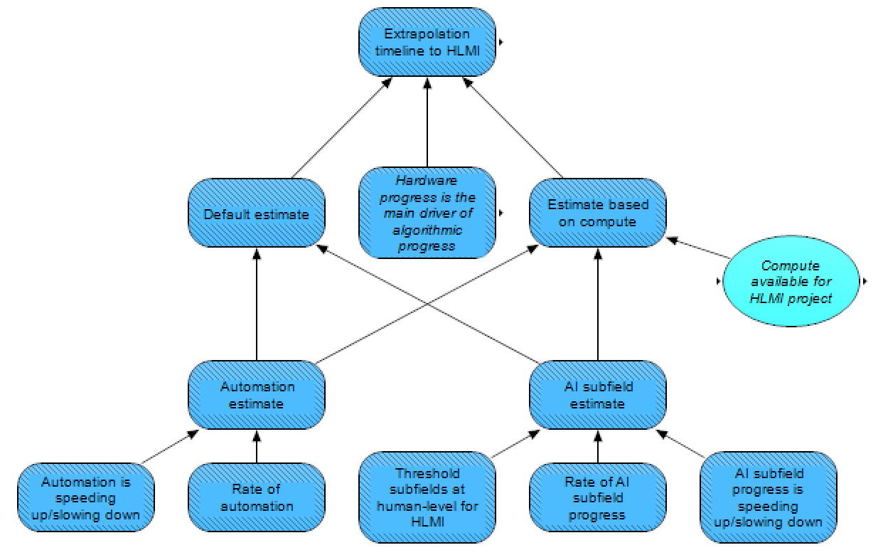
In this module, HLMI arrival is extrapolated from the rate of automation (i.e., to occur when extrapolated automation hits 100%), and from progress in various AI subfields. Such an extrapolation is perhaps particularly appropriate if one is expecting HLMI to arrive in a piecemeal fashion, with different AIs highly specialized for automating specific tasks in a larger economy. Note that questions about the distribution versus concentration of HLMI are handled by a downstream module in our model, covered in a subsequent post.
For the extrapolation from automation, this calculation depends on the rate of automation, and whether this rate has generally been speeding up, slowing down, or remaining roughly constant.
For the extrapolation from the progress in various AI subfields, a somewhat similar calculation is performed, considering again the rate of progress and whether this progress has been speeding up, slowing down, or remaining roughly constant. HLMI is assumed to be achieved here when enough subfields are extrapolated to reach human-level performance.
One crux for this calculation, however, is the threshold for what portion of subfields need to reach human level in the extrapolation to reach HLMI. One could imagine that all subfields may need to reach human level, as HLMI wouldn’t be achieved until AI was as good as humans in all these subfields, but this threshold would introduce a couple problems. First, if certain subfields happen to be dominated by researchers that are more conservative in their estimations, then the most pessimistic subfield could bias the results to be too conservative. Second, it’s possible that some subfields are bottlenecked by sufficient success in other subfields, and will see very slow progress before these other subfields reach sufficient capabilities. Alternatively, one could imagine that the response from the median subfield may be the least biased, and also be the most appropriate for gauging “general” intelligence. On the other hand, if AI achieving human-level competence on half of the domains did not translate into similar competence in other domains, then this would not imply HLMI.
Similar to the above section on analogies to other developments, the extrapolation here is done in two forms: as a default case, it is performed in terms of time, but if hardware progress is the main driver of algorithmic progress, then the extrapolation is performed in terms of (the logarithm of) compute. In the latter scenario, a slowdown in compute would lead to a comparable slowdown in AI capability gains, all else equal.
Bringing it all together
Here, we have examined several methods for estimating the timeline to HLMI: a gears-level model of specific pathways to HLMI, as well as analogizing HLMI to other developments in plausibly similar reference classes, and additionally extrapolating current trends in automation and AI progress. Disagreements exist regarding the proper weight for these different forecasting methods, and further disagreements exist for many factors underlying these estimations, including some factors that appear in several different places (e.g., the progression of hardware and cruxes related to analogies and general priors on intelligence [? · GW]).
In addition to estimating the timeline to HLMI, our model also allows for estimating the method of HLMI first achieved – though such an estimate only occurs in one of our three forecasting methods (we welcome suggestions for how to make this estimate in model runs where other methods are “chosen” by the Monte Carlo method dice roll, as this information is important for downstream nodes in other parts of our model).
In the next post in this series, we will discuss AI takeoff speeds and discontinuities around and after HLMI.
Acknowledgments
We would like to thank both the rest of the MTAIR project team [? · GW], as well as the following individuals, for valuable feedback on this post: Edo Arad, Lukas Finnveden, Ozzie Gooen, Jennifer Lin, Rohin Shah, and Ben Snodin
9 comments
Comments sorted by top scores.
comment by Daniel Kokotajlo (daniel-kokotajlo) · 2021-09-26T11:16:31.341Z · LW(p) · GW(p)
I think this sequence of posts is underrated/underappreciated. I think this is because (A) it's super long and dense and (B) mostly a summary/distillation/textbook thingy rather than advancing new claims or arguing for something controversial. As a result of (a) and (b) perhaps it struggles to hold people's attention all the way through.
But that's a shame because this sort of project seems pretty useful to me. It seems like the community should be throwing money and interns at you, so that you can build a slick interactive website that displays the full graph (perhaps with expandable/collapsible subsections) and has the relevant paragraphs of text appear when you hover over each node, and that would just be Phase 1, Phase 2 would be adding mathematical relationships to the links and numbers to the nodes, such that people can input their own numbers and the whole system updates itself to spit out answers about nodes at the end. The end result would be like a wiki + textbook only better organized and more fun, while simultaneously being a the most detailed and comprehensive quantitative model of AI stuff ever.
Replies from: alenglander↑ comment by Aryeh Englander (alenglander) · 2021-09-26T11:52:33.783Z · LW(p) · GW(p)
Thanks Daniel for that strong vote of confidence!
The full graph is in fact expandable / collapsible, and it does have the ability to display the relevant paragraphs when you hover over a node (although the descriptions are not all filled in yet). It also allows people to enter in their own numbers and spit out updated calculations, exactly as you described. We actually built a nice dashboard for that - we haven't shown it yet in this sequence because this sequence is mostly focused on phase 1 and that's for phase 2.
Analytica does have a web version, but it's a bit clunky and buggy so we haven't used it so far. However, I was just informed that they are coming out with a major update soon that will include a significantly better web version, so hopefully we can do all this then.
I certainly don't think we'd say no to additional funding or interns! We could certainly use them - there are quite a few areas that we have not looked into sufficiently because all of our team members were focused on other parts of the model. And we haven't gotten yet to much of the quantitative part (phase 2 as you called it), or the formal elicitation part.
Replies from: dsj↑ comment by dsj · 2022-12-27T20:35:20.224Z · LW(p) · GW(p)
Thank you for this resource, which I've been reading through!
Is there a link to the expandable/collapsible version of the full graph, or alternatively an image of the full graph which is in high enough resolution to be able to clearly read the text of the individual nodes? (I haven't found such a thing anywhere in this LW sequence or the PDF on arXiv, but maybe I missed it.)
comment by Steven Byrnes (steve2152) · 2021-09-10T15:38:14.513Z · LW(p) · GW(p)
This is great! Here's a couple random thoughts:
Hybrid statistical-symbolic HLMI
I think there's a common habit of conflating "symbolic" with "not brute force" and "not bitter lesson" but that it's not right. For example, if I were to write an algorithm that takes a ton of unstructured data and goes off and builds a giant PGM that best explains all that data, I would call that a "symbolic" AI algorithm (because PGMs are kinda discrete / symbolic / etc.), but I would also call it a "statistical" AI algorithm, and I would certainly call it "compatible with The Bitter Lesson".
(Incidentally, this description is pretty close to my oversimplified caricature description of what the neocortex does.)
(I'm not disputing that "symbolic" and "containing lots of handcrafted domain-specific structure" do often go together in practice today—e.g. Josh Tenenbaum's papers tend to have both and OpenAI papers tend to have neither—I'm just saying they don't necessarily go together.)
I don't have a concrete suggestion of what if anything you should change here, I'm just chatting. :-)
Cognitive-science approach
This is all fine except that I kinda don't like the term "cognitive science" for what you're talking about. Maybe it's just me, but anyway here's where I'm coming from:
Learning algorithms almost inevitably have the property that the trained models are more complex than the learning rules that create them. For example, compare the code to run gradient descent and train a ConvNet (it's not very complicated) to the resulting image-classification algorithms as explored in the OpenAI microscope project (they're much more complicated).
I bring this up because "cognitive science" to me has a connotation of "the study of how human brains do all the things that human brains do", especially adult human brains. After all, that's the main thing that most cognitive scientists study AFAICT. So if you think that human intelligence is "mostly a trained model", then you would think that most cognitive science is "mostly akin to OpenAI microscope" as opposed to "mostly akin to PyTorch", and therefore mostly unnecessary and unhelpful for building HLMI. You don't have to think that—certainly Gary Marcus & Steven Pinker don't—but I do (to a significant extent) and at least a few other prominent neuroscientists do too (e.g. Randall O'Reilly). (See "learning-from-scratch-ism" section here [LW · GW], also cortical uniformity here [LW · GW].) So as much as I buy into (what you call) "the cognitive-science approach", I'm not just crazy about that term, and for my part I prefer to talk about "brain algorithms" or "high-level brain algorithms". I think "brain algorithms" is more agnostic about the nature of the algorithms, and in particular whether it's the kinds of algorithms that neuroscientists talk about, versus the kinds of algorithms that computational cognitive scientists & psychologists talk about.
Replies from: Daniel_Eth↑ comment by Daniel_Eth · 2021-09-12T12:52:22.656Z · LW(p) · GW(p)
Thanks!
I agree that symbolic doesn't have to mean not bitter lesson-y (though in practice I think there are often effects in that direction). I might even go a bit further than you here and claim that a system with a significant amount of handcrafted aspects might still be bitter lesson-y, under the right conditions. The bitter lesson doesn't claim that the maximally naive and brute-force method possible will win, but instead that, among competing methods, more computationally-scalable methods will generally win over time (as compute increases). This shouldn't be surprising, as if methods A and B were both appealing enough to receive attention to begin with, then as compute increases drastically, we'd expect the method of the two that was more compute-leveraging to pull ahead. This doesn't mean that a different method C, which was more naive/brute-force than either A or B, but wasn't remotely competitive with A and B to begin with, would also pull ahead. Also, insofar as people are hardcoding in things that do scale well with compute (maybe certain types of biases, for instance), that may be more compatible with the bitter lesson than, say, hardcoding in domain knowledge.
Part of me also wonders what happens to the bitter lesson if compute really levels off. In such a world, the future gains from leveraging further compute don't seem as appealing, and it's possible larger gains can be had elsewhere.
comment by Quintin Pope (quintin-pope) · 2021-09-10T20:08:16.350Z · LW(p) · GW(p)
Thank you for this excellent post. Here are some thoughts I had while reading.
The hard paths hypothesis:
I think there's another side to the hard paths hypothesis. We are clearly the first technology-using species to evolve on Earth. However, it's entirely possible that we're not the first species with human-level intelligence. If a species with human level intelligence but no opposable thumbs evolved millions of years ago, they could have died out without leaving any artifacts we'd recognize as signs of intelligence.
Besides our intelligence, humans seem odd in many ways that could plausibly contribute to developing a technological civilization.
- We are pretty long-lived.
- We are fairly social.
- Feral children raised outside of human culture experience serious and often permanent mental disabilities (Wikipedia).
- A species with human-level intelligence, but whose members live mostly independently may not develop technological civilization.
- We have very long childhoods.
- We have ridiculously high manual dexterity (even compared to other primates).
- We live on land.
- Most animals are aquatic.
- It's hard to have an industrial revolution when you can't burn things.
- Note that by Wikipedia's listed estimates for cortical neuron counts, there are multiple dolphin/whale species with higher counts than us.
Given how well-tuned our biology seems for developing civilization, I think it's plausible that multiple human-level intelligent species arose in Earth's history, but additional bottlenecks prevented them from developing technological civilization. However, most of these bottlenecks wouldn't be an issue for an intelligence generated by simulated evolution. E.g., we could intervene in such a simulation to give low-dexterity species other means of manipulating their environment. Perhaps Earth's evolutionary history actually contains n human-level intelligent species, only one of which developed technology. That implies the true compute required to evolve human-level intelligence is far lower.
Brain imitation learning:
I also think the discussion of neuromophic AI and whole brain emulation misses an important possibility that Gwern calls "brain imitation learning". In essence, you record a bunch of data about human brain activity (using EEG, implanted electrodes, etc.), then you train a deep neural network to model the recorded data (similar to how GPT-3 or BERT model text). The idea is that modeling brain activity will cause the deep network to learn some of the brain's neurological algorithms. Then, you train the deep network on some downstream task and hope its learned brain algorithms generalize to the task in question.
I think brain imitation learning is pretty likely to work. We've repeatedly seen in deep learning that knowledge distillation (training a smaller student model to imitate a larger teacher model) is FAR more computationally efficient than trying to train the student model from scratch, while also giving superior performance (Wikipedia, distilling BERT, distilling CLIP). Admittedly, brain activity data is pretty expensive. However, the project that finally builds human-level AI will plausibly cost billions of dollars in compute for training. If brain imitation learning can cut the price by even 10%, it will be worth hundreds of millions in terms of saved compute costs.
Replies from: Daniel_Eth↑ comment by Daniel_Eth · 2021-09-12T13:49:50.853Z · LW(p) · GW(p)
Thanks for the comments!
Re: The Hard Paths Hypothesis
I think it's very unlikely that Earth has seen other species as intelligent as humans (with the possible exception of other Homo species). In short, I suspect there is strong selection pressure for (at least many of) the different traits that allow humans to have civilization to go together. Consider dexterity – such skills allow one to use intelligence to make tools; that is, the more dexterous one is, the greater the evolutionary value of high intelligence, and the more intelligent one is, the greater the evolutionary value of dexterity. Similar positive feedback loops also seem likely between intelligence and: longevity, being omnivorous, having cumulative culture, hypersociality, language ability, vocal control, etc.
Regarding dolphins and whales, it is true that many have more neurons than us, but they also have thin cortices, low neuronal packing densities, and low axonal conduction velocities (in addition to lower EQs than humans).
Additionally, birds and mammals are both considered unusually intelligent for animals (more so than reptiles, amphibians, fish, etc), and both birds and mammals have seen (neurological evidence of) gradual trends of increasing (maximum) intelligence over the course of the past 100 MY or more (and even extant nonhuman great apes seem most likely to be somewhat smarter than their last common ancestors with humans). So if there was a previously intelligent species, I'd be scratching my head about when it would have evolved. While we can't completely rule out a previous species as smart as humans (we also can't completely rule out a previous technological species, for which all artifacts have been destroyed), I think the balance of evidence is pretty strongly against, though I'll admit that not everyone shares this view. Personally, I'd be absolutely shocked if there were 10+ (not very closely related) previous intelligent species, which is what would be required to reduce compute by just 1 OOM. (And even then, insofar as the different species shared a common ancestor, there still could be a hard step that the ancestor passed.)
But I do think it's the case that certain bottlenecks on Earth wouldn't be a bottleneck for engineers. For instance, I think there's a good chance that we simply got lucky in the past several hundred million years for the climate staying ~stable instead of spiraling into uninhabitable hothouse or snowball states (i.e., we may be subject to survivorship bias here); this seems very easy for human engineers to work around in simulations. The same is plausibly true for other bottlenecks as well.
Re: Brain imitation learning
My cop-out answer here is that this is already covered by the "other methods" section. My real answer is that the model isn't great at handling approaches that are intermediate between different methods. I agree it makes sense to continue to watch this space.
comment by Davidmanheim · 2021-09-11T17:57:17.887Z · LW(p) · GW(p)
On the topic of growth rate of computing power, it's worth noting that we expect the model which experts have to be somewhat more complex that what we represented as "Moore's law through year " - but as with the simplification regarding CPU/GPU/ASIC compute, I'm unsure how much this is really a crux for anyone about the timing for AGI.
I would be very interested to hear from anyone who said, for example, "I would expect AGI by 2035 if Moore's law continues, but I expect it to end before 2030, and it will therefore likely take until 2050 to reach HLMI/AGI."
↑ comment by Daniel_Eth · 2021-09-12T12:17:38.723Z · LW(p) · GW(p)
I think very few people would explicitly articulate a view like that, but I also think there are people who hold a view along the lines of, "Moore will continue strong for a number of years, and then after that compute/$ will grow at <20% as fast" – in which case, if we're bottlenecked on hardware, whether Moore ends several years earlier vs later could have a large effect on timelines.